15 853 Algorithms in the Real World Locality

15 -853: Algorithms in the Real World Locality II: Cache-oblivious algorithms – Matrix multiplication – Distribution sort – Static searching

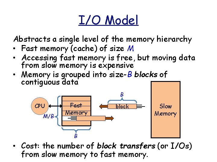
I/O Model Abstracts a single level of the memory hierarchy • Fast memory (cache) of size M • Accessing fast memory is free, but moving data from slow memory is expensive • Memory is grouped into size-B blocks of contiguous data B CPU M/B Fast Memory block Slow Memory B • Cost: the number of block transfers (or I/Os) from slow memory to fast memory.

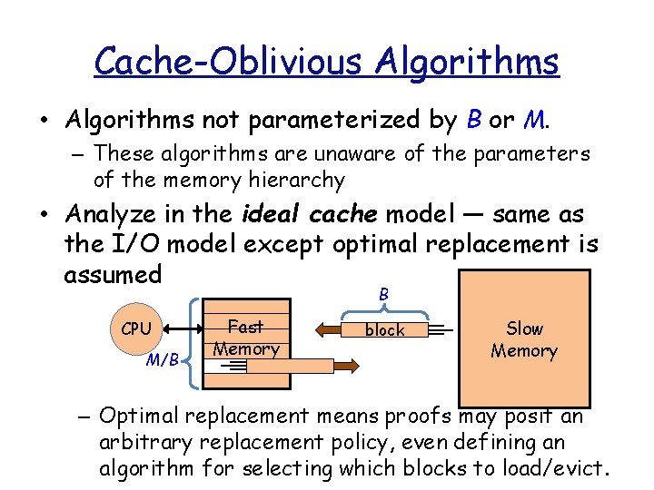
Cache-Oblivious Algorithms • Algorithms not parameterized by B or M. – These algorithms are unaware of the parameters of the memory hierarchy • Analyze in the ideal cache model — same as the I/O model except optimal replacement is assumed B CPU M/B Fast Memory block Slow Memory – Optimal replacement means proofs may posit an arbitrary replacement policy, even defining an algorithm for selecting which blocks to load/evict.

Advantages of Cache-Oblivious Algorithms • Since CO algorithms do not depend on memory parameters, bounds generalize to multilevel hierarchies. • Algorithms are platform independent • Algorithms should be effective even when B and M are not static

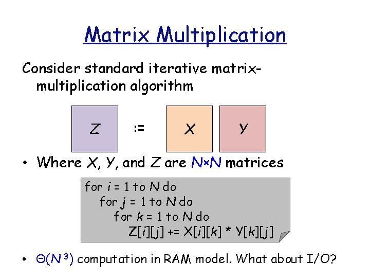
Matrix Multiplication Consider standard iterative matrixmultiplication algorithm Z : = X Y • Where X, Y, and Z are N×N matrices for i = 1 to N do for j = 1 to N do for k = 1 to N do Z[i][j] += X[i][k] * Y[k][j] • Θ(N 3) computation in RAM model. What about I/O?

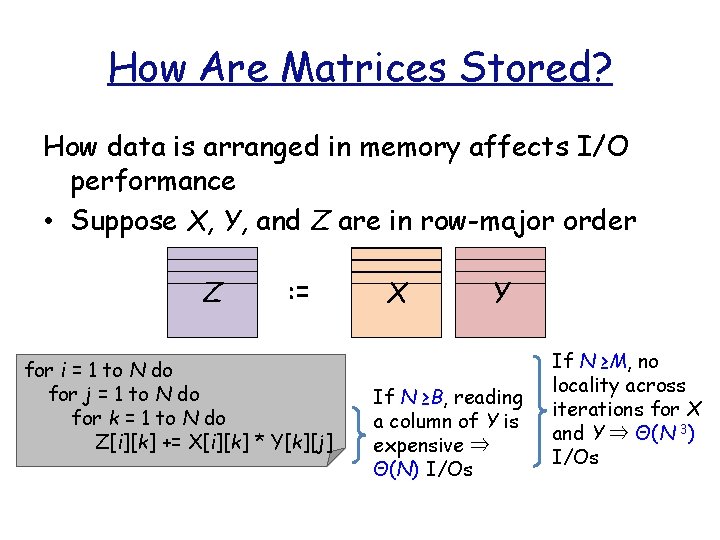
How Are Matrices Stored? How data is arranged in memory affects I/O performance • Suppose X, Y, and Z are in row-major order Z : = for i = 1 to N do for j = 1 to N do for k = 1 to N do Z[i][k] += X[i][k] * Y[k][j] X Y If N ≥B, reading a column of Y is expensive ⇒ Θ(N) I/Os If N ≥M, no locality across iterations for X and Y ⇒ Θ(N 3) I/Os

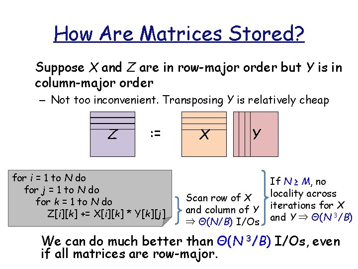
How Are Matrices Stored? Suppose X and Z are in row-major order but Y is in column-major order – Not too inconvenient. Transposing Y is relatively cheap Z : = for i = 1 to N do for j = 1 to N do for k = 1 to N do Z[i][k] += X[i][k] * Y[k][j] X Y Scan row of X and column of Y ⇒ Θ(N/B) I/Os If N ≥ M, no locality across iterations for X and Y ⇒ Θ(N 3/B) We can do much better than Θ(N 3/B) I/Os, even if all matrices are row-major.

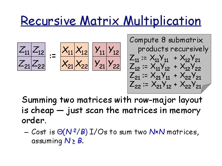
Recursive Matrix Multiplication Z 11 Z 12 Z 21 Z 22 : = X 11 X 12 Y 11 Y 12 X 21 X 22 Y 21 Y 22 Compute 8 submatrix products recursively Z 11 : = X 11 Y 11 + X 12 Y 21 Z 12 : = X 11 Y 12 + X 12 Y 22 Z 21 : = X 21 Y 11 + X 22 Y 21 Z 22 : = X 21 Y 12 + X 22 Y 21 Summing two matrices with row-major layout is cheap — just scan the matrices in memory order. – Cost is Θ(N 2/B) I/Os to sum two N×N matrices, assuming N ≥ B.

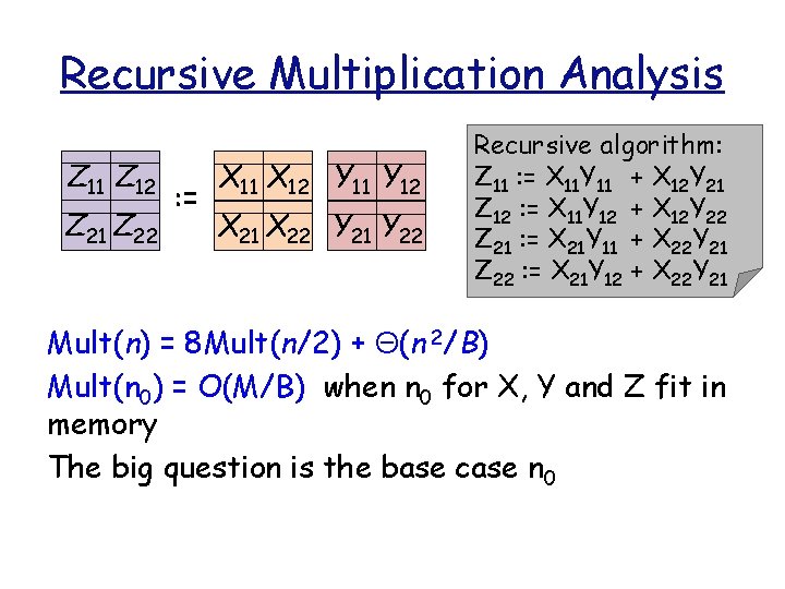
Recursive Multiplication Analysis Z 11 Z 12 Z 21 Z 22 : = X 11 X 12 Y 11 Y 12 X 21 X 22 Y 21 Y 22 Recursive algorithm: Z 11 : = X 11 Y 11 + X 12 Y 21 Z 12 : = X 11 Y 12 + X 12 Y 22 Z 21 : = X 21 Y 11 + X 22 Y 21 Z 22 : = X 21 Y 12 + X 22 Y 21 Mult(n) = 8 Mult(n/2) + Θ(n 2/B) Mult(n 0) = O(M/B) when n 0 for X, Y and Z fit in memory The big question is the base case n 0

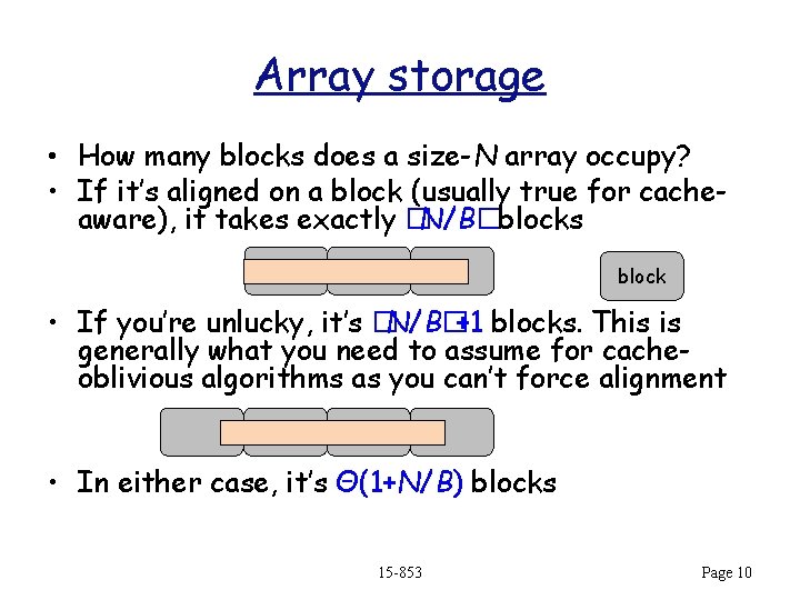
Array storage • How many blocks does a size-N array occupy? • If it’s aligned on a block (usually true for cacheaware), it takes exactly �N/B�blocks block • If you’re unlucky, it’s �N/B�+1 blocks. This is generally what you need to assume for cacheoblivious algorithms as you can’t force alignment • In either case, it’s Θ(1+N/B) blocks 15 -853 Page 10

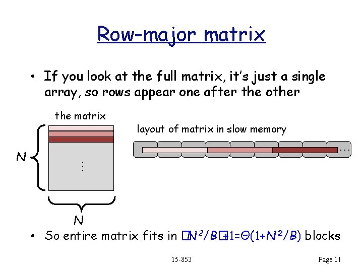
Row-major matrix • If you look at the full matrix, it’s just a single array, so rows appear one after the other the matrix … … N layout of matrix in slow memory N • So entire matrix fits in �N 2/B�+1=Θ(1+N 2/B) blocks 15 -853 Page 11

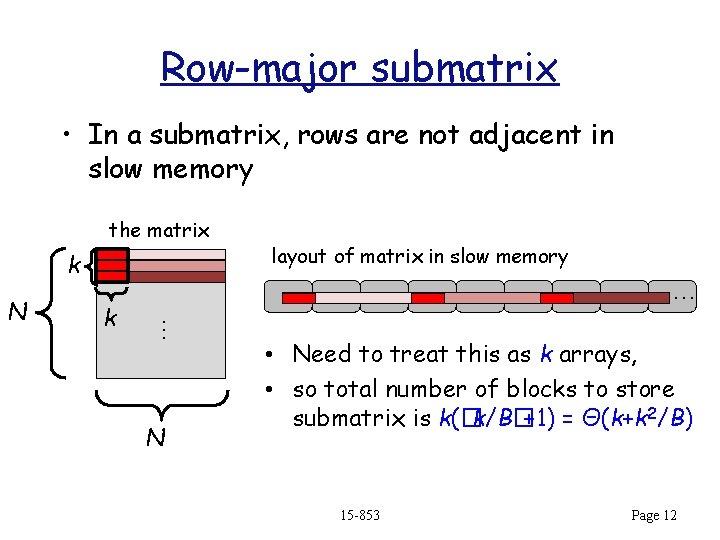
Row-major submatrix • In a submatrix, rows are not adjacent in slow memory the matrix k k … … N layout of matrix in slow memory N • Need to treat this as k arrays, • so total number of blocks to store submatrix is k(�k/B� +1) = Θ(k+k 2/B) 15 -853 Page 12

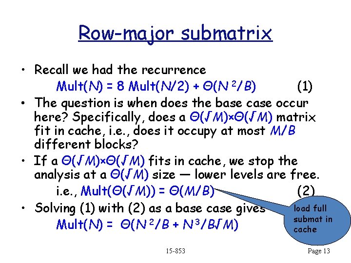
Row-major submatrix • Recall we had the recurrence Mult(N) = 8 Mult(N/2) + Θ(N 2/B) (1) • The question is when does the base case occur here? Specifically, does a Θ(√M)×Θ(√M) matrix fit in cache, i. e. , does it occupy at most M/B different blocks? • If a Θ(√M)×Θ(√M) fits in cache, we stop the analysis at a Θ(√M) size — lower levels are free. i. e. , Mult(Θ(√M)) = Θ(M/B) (2) load full • Solving (1) with (2) as a base case gives submat in 2 3 Mult(N) = Θ(N /B + N /B√M) cache 15 -853 Page 13

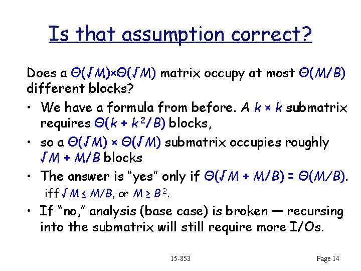
Is that assumption correct? Does a Θ(√M)×Θ(√M) matrix occupy at most Θ(M/B) different blocks? • We have a formula from before. A k × k submatrix requires Θ(k + k 2/B) blocks, • so a Θ(√M) × Θ(√M) submatrix occupies roughly √M + M/B blocks • The answer is “yes” only if Θ(√M + M/B) = Θ(M/B). iff √M ≤ M/B, or M ≥ B 2. • If “no, ” analysis (base case) is broken — recursing into the submatrix will still require more I/Os. 15 -853 Page 14

Fixing the base case Two fixes: 1. The “tall cache” assumption: M≥B 2. Then the base case is correct, completing the analysis. 2. Change the matrix layout. 15 -853 Page 15

Without Tall-Cache Assumption Try a better matrix layout • The algorithm is recursive. Use a layout that matches the recursive nature of the algorithm • For example, Z-morton ordering: - The line connects elements that are adjacent in memory - In other words, construct the layout by storing each quadrant of the matrix contiguously, and recurse

Recursive Mat. Mul with Z-Morton The analysis becomes easier • Each quadrant of the matrix is contiguous in memory, so a c√M ×c√M submatrix fits in memory – The tall-cache assumption is not required to make this base case work • The rest of the analysis is the same

Searching: binary search is bad A B C D E F G H I J K L M N O Example: binary search for element A with block size B = 2 • Search hits a a different block until reducing keyspace to size Θ(B). • Thus, total cost is log 2 N – Θ(log 2 B) = Θ(log 2(N/B)) ≈ Θ(log 2 N) for N >>B

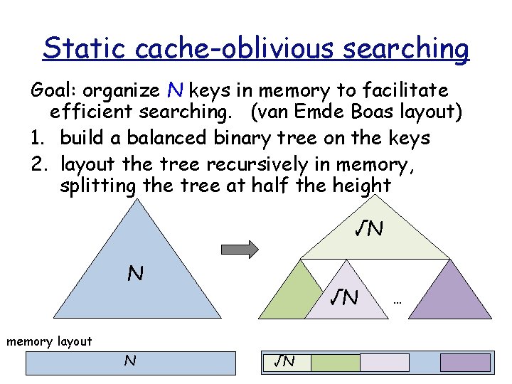
Static cache-oblivious searching Goal: organize N keys in memory to facilitate efficient searching. (van Emde Boas layout) 1. build a balanced binary tree on the keys 2. layout the tree recursively in memory, splitting the tree at half the height √N N √N memory layout N √N …

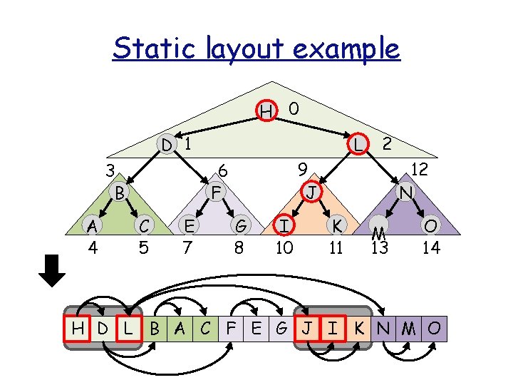
Static layout example H 0 D 1 3 B A 4 L 9 J 6 F C 5 E 7 2 G 8 I 10 12 N K 11 M 13 O 14 H D L B A C F E G J I K N M O

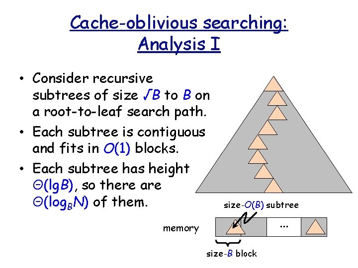
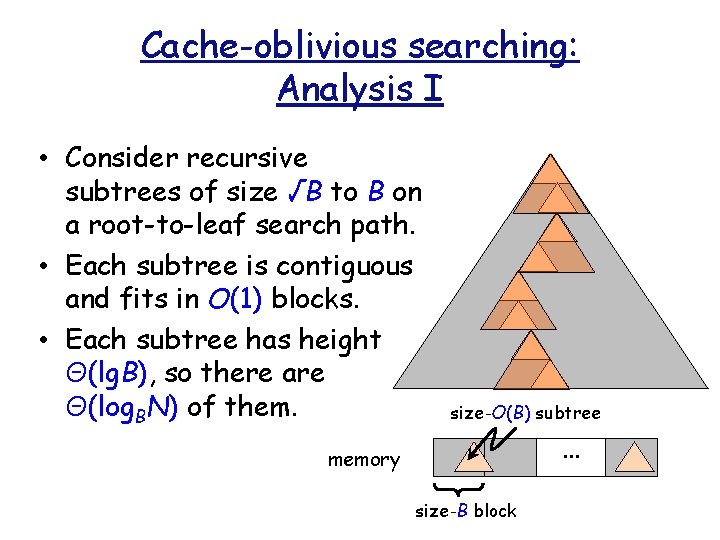
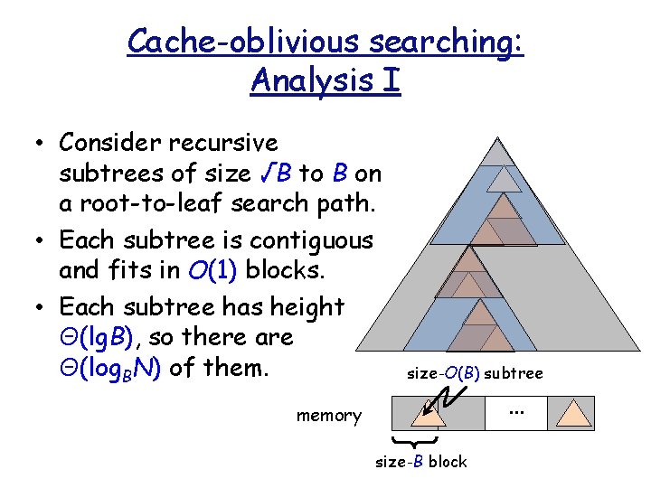
Cache-oblivious searching: Analysis I • Consider recursive subtrees of size √B to B on a root-to-leaf search path. • Each subtree is contiguous and fits in O(1) blocks. • Each subtree has height Θ(lg. B), so there are Θ(log. BN) of them. size-O(B) subtree memory size-B block …

Cache-oblivious searching: Analysis I • Consider recursive subtrees of size √B to B on a root-to-leaf search path. • Each subtree is contiguous and fits in O(1) blocks. • Each subtree has height Θ(lg. B), so there are Θ(log. BN) of them. size-O(B) subtree memory size-B block …

Cache-oblivious searching: Analysis I • Consider recursive subtrees of size √B to B on a root-to-leaf search path. • Each subtree is contiguous and fits in O(1) blocks. • Each subtree has height Θ(lg. B), so there are Θ(log. BN) of them. size-O(B) subtree memory size-B block …

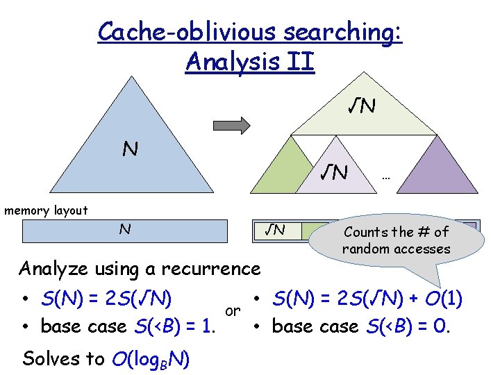
Cache-oblivious searching: Analysis II √N N √N … memory layout N Analyze using a recurrence √N Counts the # of random accesses • S(N) = 2 S(√N) + O(1) • S(N) = 2 S(√N) or • base case S(<B) = 0. • base case S(<B) = 1. Solves to O(log. BN)

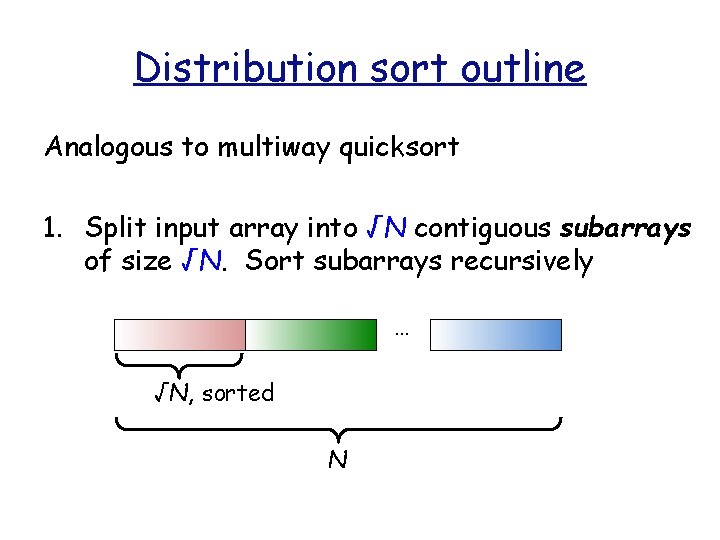
Distribution sort outline Analogous to multiway quicksort 1. Split input array into √N contiguous subarrays of size √N. Sort subarrays recursively … √N, sorted N

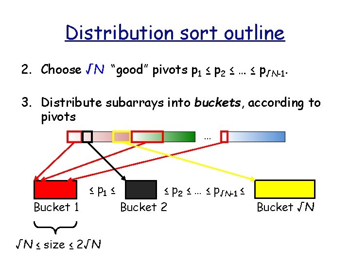
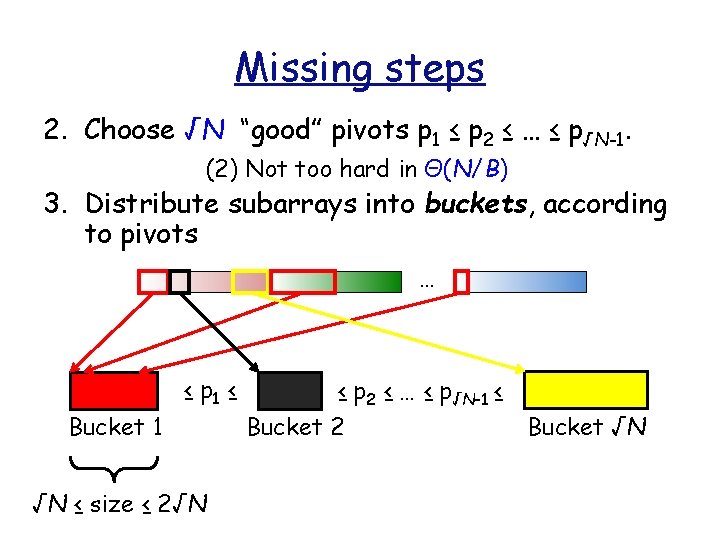
Distribution sort outline 2. Choose √N “good” pivots p 1 ≤ p 2 ≤ … ≤ p√N-1. 3. Distribute subarrays into buckets, according to pivots … Bucket 1 ≤ p 1 ≤ √N ≤ size ≤ 2√N ≤ p 2 ≤ … ≤ p√N-1 ≤ Bucket 2 Bucket √N

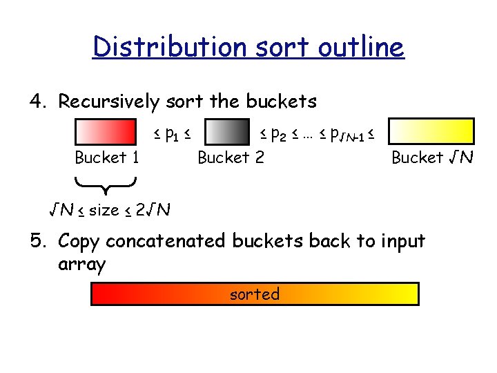
Distribution sort outline 4. Recursively sort the buckets Bucket 1 ≤ p 1 ≤ ≤ p 2 ≤ … ≤ p√N-1 ≤ Bucket 2 Bucket √N √N ≤ size ≤ 2√N 5. Copy concatenated buckets back to input array sorted

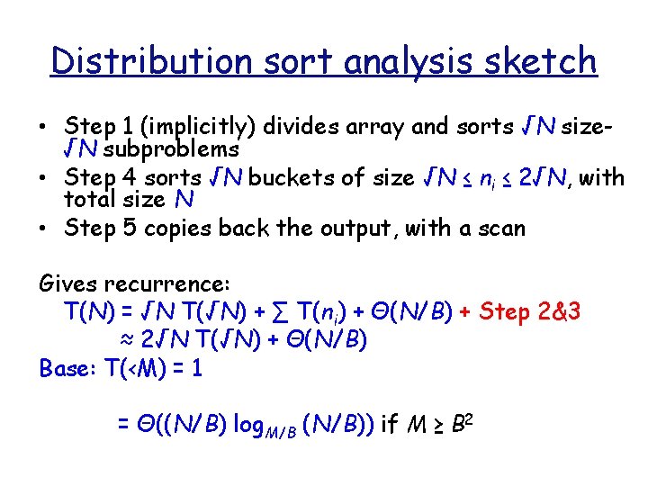
Distribution sort analysis sketch • Step 1 (implicitly) divides array and sorts √N size√N subproblems • Step 4 sorts √N buckets of size √N ≤ ni ≤ 2√N, with total size N • Step 5 copies back the output, with a scan Gives recurrence: T(N) = √N T(√N) + ∑ T(ni) + Θ(N/B) + Step 2&3 ≈ 2√N T(√N) + Θ(N/B) Base: T(<M) = 1 = Θ((N/B) log. M/B (N/B)) if M ≥ B 2

Missing steps 2. Choose √N “good” pivots p 1 ≤ p 2 ≤ … ≤ p√N-1. (2) Not too hard in Θ(N/B) 3. Distribute subarrays into buckets, according to pivots … Bucket 1 ≤ p 1 ≤ √N ≤ size ≤ 2√N ≤ p 2 ≤ … ≤ p√N-1 ≤ Bucket 2 Bucket √N

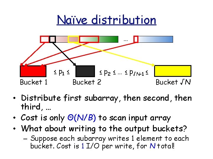
Naïve distribution … Bucket 1 ≤ p 1 ≤ ≤ p 2 ≤ … ≤ p√N-1 ≤ Bucket 2 Bucket √N • Distribute first subarray, then second, then third, … • Cost is only Θ(N/B) to scan input array • What about writing to the output buckets? – Suppose each subarray writes 1 element to each bucket. Cost is 1 I/O per write, for N total!

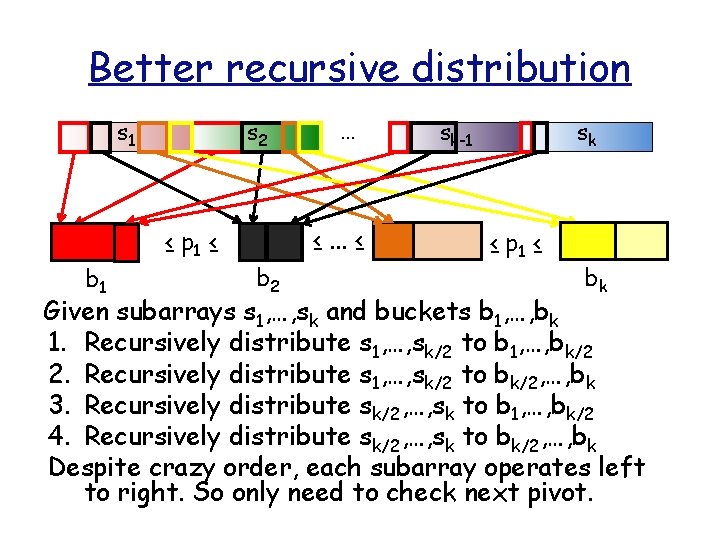
Better recursive distribution s 1 b 1 s 2 ≤ p 1 ≤ … ≤…≤ b 2 sk sk-1 ≤ p 1 ≤ bk Given subarrays s 1, …, sk and buckets b 1, …, bk 1. Recursively distribute s 1, …, sk/2 to b 1, …, bk/2 2. Recursively distribute s 1, …, sk/2 to bk/2, …, bk 3. Recursively distribute sk/2, …, sk to b 1, …, bk/2 4. Recursively distribute sk/2, …, sk to bk/2, …, bk Despite crazy order, each subarray operates left to right. So only need to check next pivot.

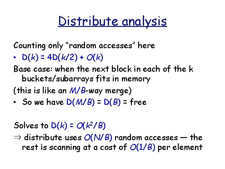
Distribute analysis Counting only “random accesses” here • D(k) = 4 D(k/2) + O(k) Base case: when the next block in each of the k buckets/subarrays fits in memory (this is like an M/B-way merge) • So we have D(M/B) = D(B) = free Solves to D(k) = O(k 2/B) ⇒ distribute uses O(N/B) random accesses — the rest is scanning at a cost of O(1/B) per element

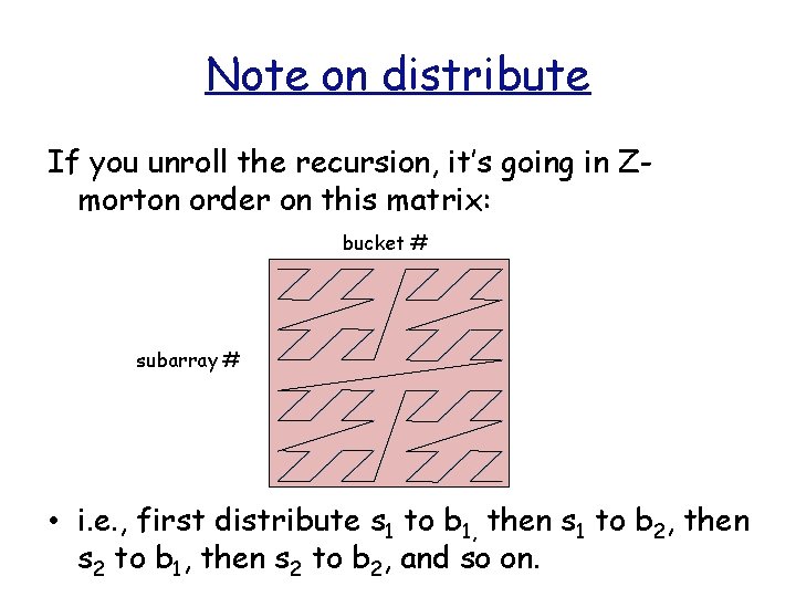
Note on distribute If you unroll the recursion, it’s going in Zmorton order on this matrix: bucket # subarray # • i. e. , first distribute s 1 to b 1, then s 1 to b 2, then s 2 to b 1, then s 2 to b 2, and so on.