Trees Make Money Fast Stock Fraud Goodrich Tamassia

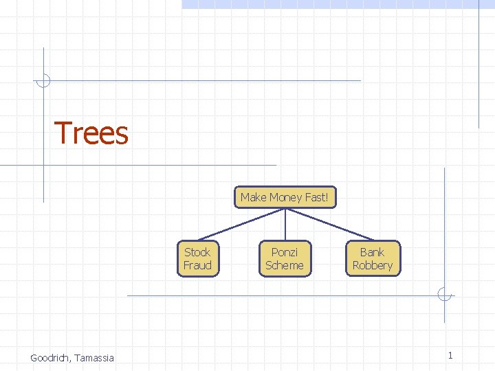
Trees Make Money Fast! Stock Fraud Goodrich, Tamassia Ponzi Scheme Bank Robbery 1

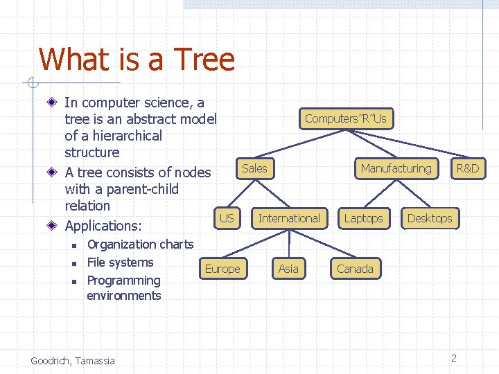
What is a Tree In computer science, a tree is an abstract model of a hierarchical structure A tree consists of nodes with a parent-child relation US Applications: n n n Organization charts File systems Europe Programming environments Goodrich, Tamassia Computers”R”Us Sales Manufacturing International Asia Laptops R&D Desktops Canada 2

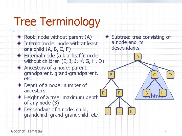
Tree Terminology Root: node without parent (A) Internal node: node with at least one child (A, B, C, F) External node (a. k. a. leaf ): node without children (E, I, J, K, G, H, D) Ancestors of a node: parent, grand-grandparent, etc. Depth of a node: number of ancestors E Height of a tree: maximum depth of any node (3) Descendant of a node: child, grand-grandchild, etc. Goodrich, Tamassia Subtree: tree consisting of a node and its descendants A B C F I J G D H subtree K 3

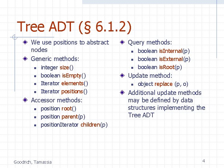
Tree ADT (§ 6. 1. 2) We use positions to abstract nodes Generic methods: n n integer size() boolean is. Empty() Iterator elements() Iterator positions() Accessor methods: n n n position root() position parent(p) position. Iterator children(p) Goodrich, Tamassia Query methods: n n n boolean is. Internal(p) boolean is. External(p) boolean is. Root(p) Update method: n object replace (p, o) Additional update methods may be defined by data structures implementing the Tree ADT 4

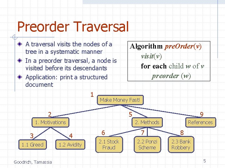
Preorder Traversal A traversal visits the nodes of a tree in a systematic manner In a preorder traversal, a node is visited before its descendants Application: print a structured document 1 Make Money Fast! 2 5 1. Motivations 9 2. Methods 3 4 1. 1 Greed 1. 2 Avidity Goodrich, Tamassia Algorithm pre. Order(v) visit(v) for each child w of v preorder (w) 6 2. 1 Stock Fraud 7 2. 2 Ponzi Scheme References 8 2. 3 Bank Robbery 5

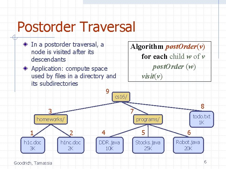
Postorder Traversal In a postorder traversal, a node is visited after its descendants Application: compute space used by files in a directory and its subdirectories 9 Algorithm post. Order(v) for each child w of v post. Order (w) visit(v) cs 16/ 3 7 homeworks/ todo. txt 1 K programs/ 1 2 h 1 c. doc 3 K h 1 nc. doc 2 K Goodrich, Tamassia 8 4 DDR. java 10 K 5 Stocks. java 25 K 6 Robot. java 20 K 6

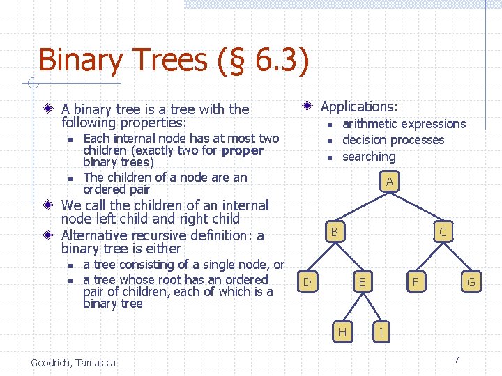
Binary Trees (§ 6. 3) Applications: A binary tree is a tree with the following properties: n n n Each internal node has at most two children (exactly two for proper binary trees) The children of a node are an ordered pair n n A We call the children of an internal node left child and right child Alternative recursive definition: a binary tree is either n n a tree consisting of a single node, or a tree whose root has an ordered pair of children, each of which is a binary tree arithmetic expressions decision processes searching B C D H Goodrich, Tamassia F E G I 7

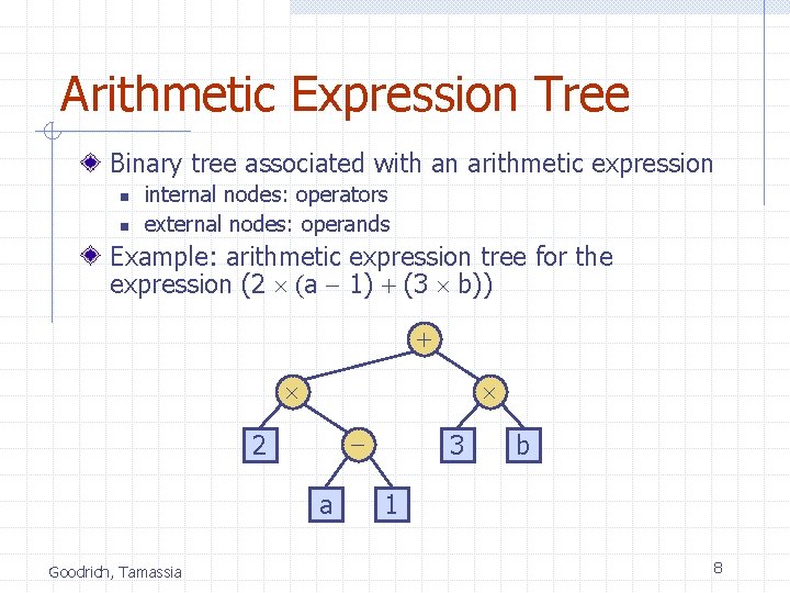
Arithmetic Expression Tree Binary tree associated with an arithmetic expression n n internal nodes: operators external nodes: operands Example: arithmetic expression tree for the expression (2 (a - 1) + (3 b)) + - 2 a Goodrich, Tamassia 3 b 1 8

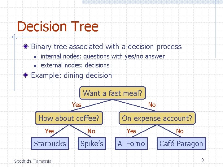
Decision Tree Binary tree associated with a decision process n n internal nodes: questions with yes/no answer external nodes: decisions Example: dining decision Want a fast meal? No Yes How about coffee? On expense account? Yes No Starbucks Spike’s Al Forno Café Paragon Goodrich, Tamassia 9

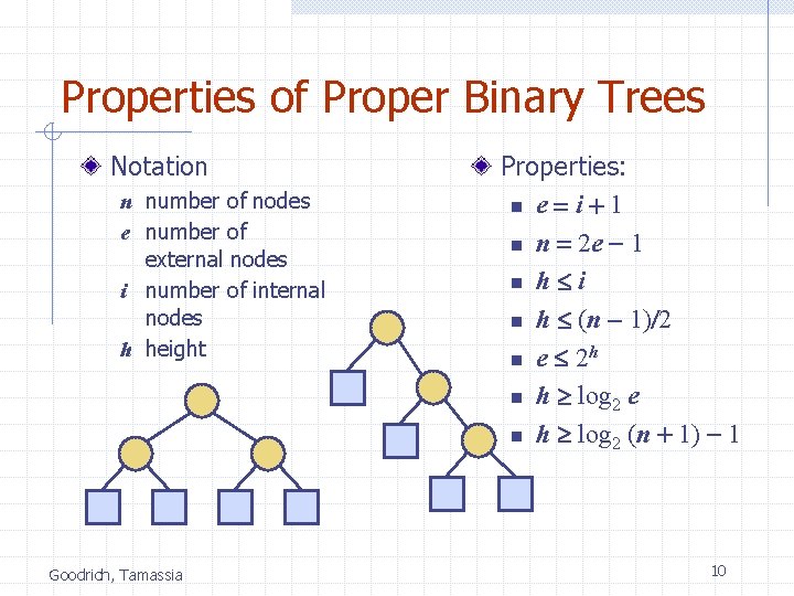
Properties of Proper Binary Trees Notation n number of nodes e number of external nodes i number of internal nodes h height Goodrich, Tamassia Properties: n e = i + 1 n n = 2 e - 1 n h i n h (n - 1)/2 n e 2 h n h log 2 e n h log 2 (n + 1) - 1 10

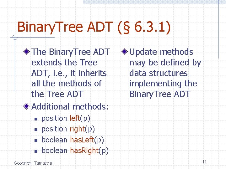
Binary. Tree ADT (§ 6. 3. 1) The Binary. Tree ADT extends the Tree ADT, i. e. , it inherits all the methods of the Tree ADT Additional methods: n n Update methods may be defined by data structures implementing the Binary. Tree ADT position left(p) position right(p) boolean has. Left(p) boolean has. Right(p) Goodrich, Tamassia 11

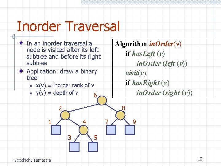
Inorder Traversal In an inorder traversal a node is visited after its left subtree and before its right subtree Application: draw a binary tree n n Algorithm in. Order(v) if has. Left (v) in. Order (left (v)) visit(v) if has. Right (v) in. Order (right (v)) x(v) = inorder rank of v y(v) = depth of v 6 2 8 1 4 3 Goodrich, Tamassia 7 9 5 12

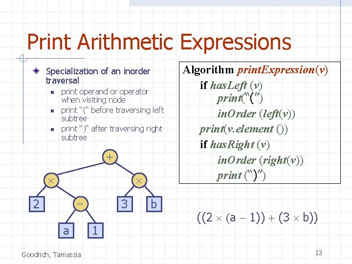
Print Arithmetic Expressions Specialization of an inorder traversal n n n print operand or operator when visiting node print “(“ before traversing left subtree print “)“ after traversing right subtree + - 2 a Goodrich, Tamassia 3 1 b Algorithm print. Expression(v) if has. Left (v) print(“(’’) in. Order (left(v)) print(v. element ()) if has. Right (v) in. Order (right(v)) print (“)’’) ((2 (a - 1)) + (3 b)) 13

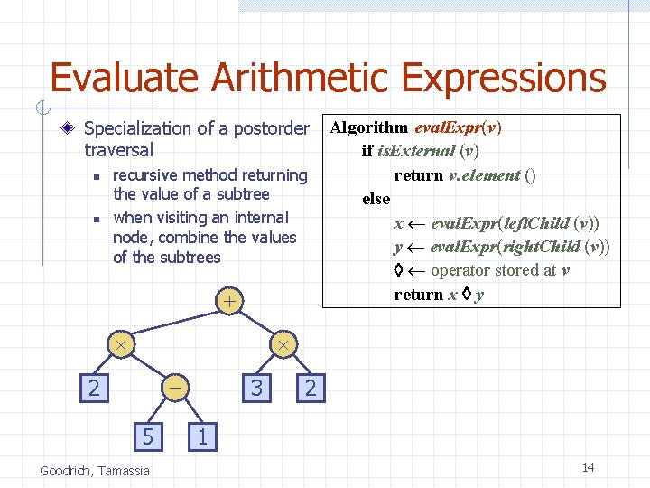
Evaluate Arithmetic Expressions Specialization of a postorder traversal n n recursive method returning the value of a subtree when visiting an internal node, combine the values of the subtrees + Algorithm eval. Expr(v) if is. External (v) return v. element () else x eval. Expr(left. Child (v)) y eval. Expr(right. Child (v)) operator stored at v return x y - 2 5 Goodrich, Tamassia 3 2 1 14

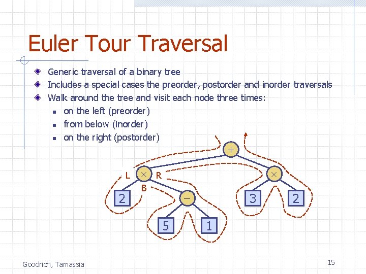
Euler Tour Traversal Generic traversal of a binary tree Includes a special cases the preorder, postorder and inorder traversals Walk around the tree and visit each node three times: n on the left (preorder) n from below (inorder) n on the right (postorder) + L 2 R B 5 Goodrich, Tamassia 3 2 1 15

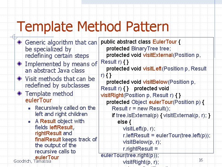
Template Method Pattern Generic algorithm that can be specialized by redefining certain steps Implemented by means of an abstract Java class Visit methods that can be redefined by subclasses Template method euler. Tour public abstract class Euler. Tour { protected Binary. Tree tree; protected void visit. External(Position p, Result r) { } protected void visit. Left(Position p, Result r) { } protected void visit. Below(Position p, Result r) { } protected void visit. Right(Position p, Result r) { } protected Object euler. Tour(Position p) { n Recursively called on the Result r = new Result(); left and right children if tree. is. External(p) { visit. External(p, r); } n A Result object with else { fields left. Result, visit. Left(p, r); right. Result and r. left. Result = euler. Tour(tree. left(p)); final. Result keeps track of visit. Below(p, r); the output of the r. right. Result = recursive calls to euler. Tour(tree. right(p)); euler. Tour 16 Goodrich, Tamassia visit. Right(p, r);

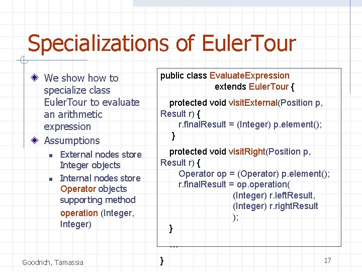
Specializations of Euler. Tour We show to specialize class Euler. Tour to evaluate an arithmetic expression Assumptions n n External nodes store Integer objects Internal nodes store Operator objects supporting method operation (Integer, Integer) public class Evaluate. Expression extends Euler. Tour { protected void visit. External(Position p, Result r) { r. final. Result = (Integer) p. element(); } protected void visit. Right(Position p, Result r) { Operator op = (Operator) p. element(); r. final. Result = op. operation( (Integer) r. left. Result, (Integer) r. right. Result ); } … Goodrich, Tamassia } 17

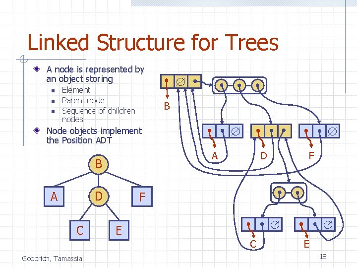
Linked Structure for Trees A node is represented by an object storing n n n Element Parent node Sequence of children nodes B Node objects implement the Position ADT A B D A C D F E C Goodrich, Tamassia F E 18

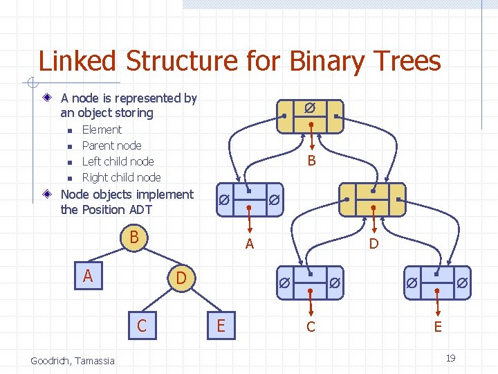
Linked Structure for Binary Trees A node is represented by an object storing n n Element Parent node Left child node Right child node B Node objects implement the Position ADT B A Goodrich, Tamassia A D C D E C E 19

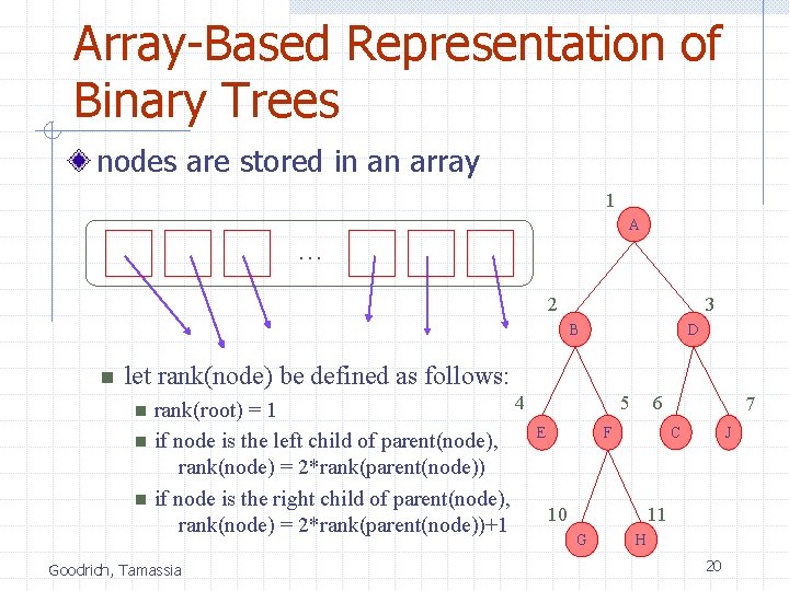
Array-Based Representation of Binary Trees nodes are stored in an array 1 A … 2 3 B n D let rank(node) be defined as follows: n n n 4 rank(root) = 1 if node is the left child of parent(node), rank(node) = 2*rank(parent(node)) if node is the right child of parent(node), rank(node) = 2*rank(parent(node))+1 Goodrich, Tamassia 5 E 6 7 C F 10 J 11 G H 20

Priority Queues Goodrich, Tamassia 21

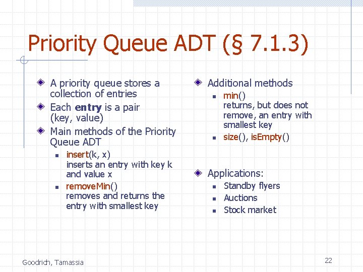
Priority Queue ADT (§ 7. 1. 3) A priority queue stores a collection of entries Each entry is a pair (key, value) Main methods of the Priority Queue ADT n n insert(k, x) inserts an entry with key k and value x remove. Min() removes and returns the entry with smallest key Goodrich, Tamassia Additional methods n n min() returns, but does not remove, an entry with smallest key size(), is. Empty() Applications: n n n Standby flyers Auctions Stock market 22

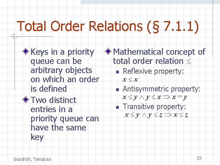
Total Order Relations (§ 7. 1. 1) Keys in a priority queue can be arbitrary objects on which an order is defined Two distinct entries in a priority queue can have the same key Goodrich, Tamassia Mathematical concept of total order relation n n n Reflexive property: x x Antisymmetric property: x y y x x=y Transitive property: x y y z x z 23

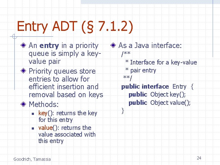
Entry ADT (§ 7. 1. 2) An entry in a priority queue is simply a keyvalue pair Priority queues store entries to allow for efficient insertion and removal based on keys Methods: n n key(): returns the key for this entry value(): returns the value associated with this entry Goodrich, Tamassia As a Java interface: /** * Interface for a key-value * pair entry **/ public interface Entry { public Object key(); public Object value(); } 24

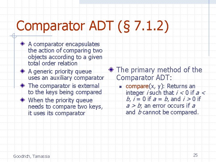
Comparator ADT (§ 7. 1. 2) A comparator encapsulates the action of comparing two objects according to a given total order relation A generic priority queue uses an auxiliary comparator The comparator is external to the keys being compared When the priority queue needs to compare two keys, it uses its comparator Goodrich, Tamassia The primary method of the Comparator ADT: n compare(x, y): Returns an integer i such that i < 0 if a < b, i = 0 if a = b, and i > 0 if a > b; an error occurs if a and b cannot be compared. 25

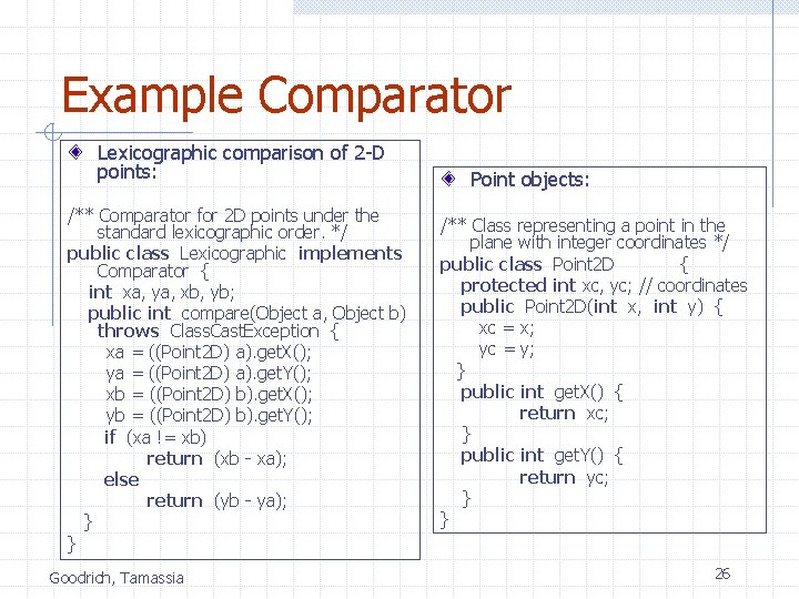
Example Comparator Lexicographic comparison of 2 -D points: /** Comparator for 2 D points under the standard lexicographic order. */ public class Lexicographic implements Comparator { int xa, ya, xb, yb; public int compare(Object a, Object b) throws Class. Cast. Exception { xa = ((Point 2 D) a). get. X(); ya = ((Point 2 D) a). get. Y(); xb = ((Point 2 D) b). get. X(); yb = ((Point 2 D) b). get. Y(); if (xa != xb) return (xb - xa); else return (yb - ya); } } Goodrich, Tamassia Point objects: /** Class representing a point in the plane with integer coordinates */ public class Point 2 D { protected int xc, yc; // coordinates public Point 2 D(int x, int y) { xc = x; yc = y; } public int get. X() { return xc; } public int get. Y() { return yc; } } 26

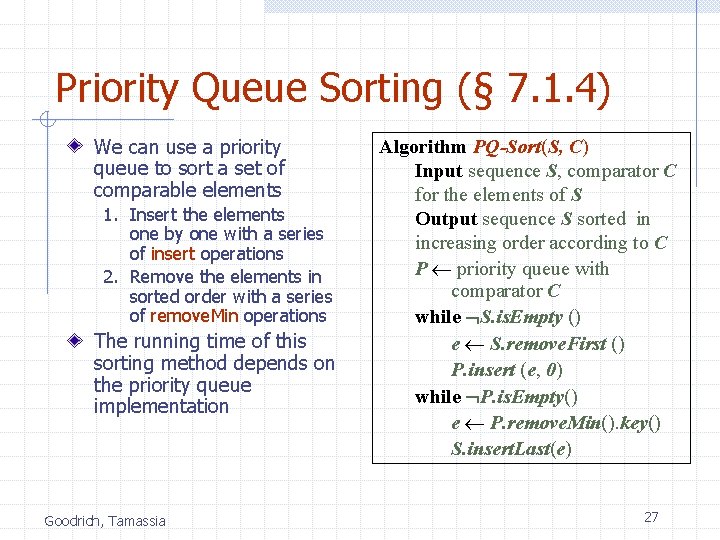
Priority Queue Sorting (§ 7. 1. 4) We can use a priority queue to sort a set of comparable elements 1. Insert the elements one by one with a series of insert operations 2. Remove the elements in sorted order with a series of remove. Min operations The running time of this sorting method depends on the priority queue implementation Goodrich, Tamassia Algorithm PQ-Sort(S, C) Input sequence S, comparator C for the elements of S Output sequence S sorted in increasing order according to C P priority queue with comparator C while S. is. Empty () e S. remove. First () P. insert (e, 0) while P. is. Empty() e P. remove. Min(). key() S. insert. Last(e) 27

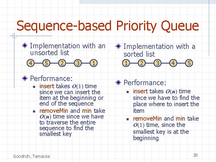
Sequence-based Priority Queue Implementation with an unsorted list Implementation with a sorted list 4 1 5 2 Performance: n n 3 1 insert takes O(1) time since we can insert the item at the beginning or end of the sequence remove. Min and min take O(n) time since we have to traverse the entire sequence to find the smallest key Goodrich, Tamassia 2 3 4 5 Performance: n n insert takes O(n) time since we have to find the place where to insert the item remove. Min and min take O(1) time, since the smallest key is at the beginning 28

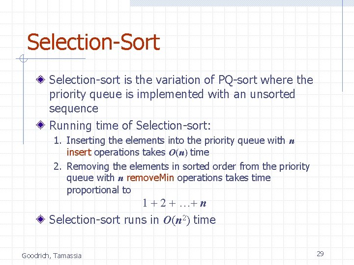
Selection-Sort Selection-sort is the variation of PQ-sort where the priority queue is implemented with an unsorted sequence Running time of Selection-sort: 1. Inserting the elements into the priority queue with n insert operations takes O(n) time 2. Removing the elements in sorted order from the priority queue with n remove. Min operations takes time proportional to 1 + 2 + …+ n Selection-sort runs in O(n 2) time Goodrich, Tamassia 29

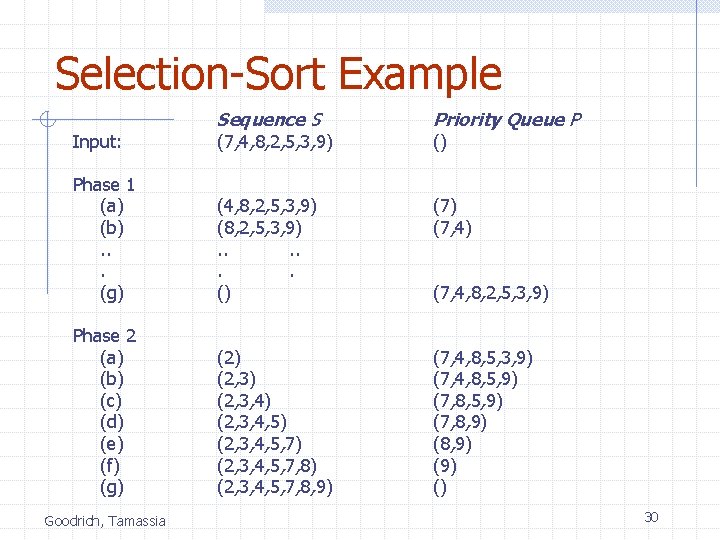
Selection-Sort Example Input: Sequence S (7, 4, 8, 2, 5, 3, 9) Priority Queue P Phase 1 (a) (b). . . (g) (4, 8, 2, 5, 3, 9) (8, 2, 5, 3, 9). . . () (7, 4) Phase 2 (a) (b) (c) (d) (e) (f) (g) (2, 3) (2, 3, 4, 5) (2, 3, 4, 5, 7, 8) (2, 3, 4, 5, 7, 8, 9) (7, 4, 8, 5, 3, 9) (7, 4, 8, 5, 9) (7, 8, 9) (9) () Goodrich, Tamassia () (7, 4, 8, 2, 5, 3, 9) 30

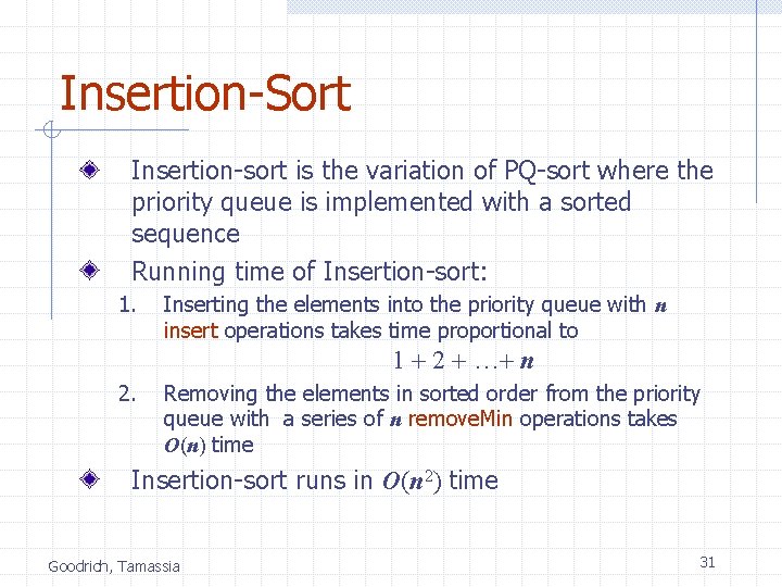
Insertion-Sort Insertion-sort is the variation of PQ-sort where the priority queue is implemented with a sorted sequence Running time of Insertion-sort: 1. Inserting the elements into the priority queue with n insert operations takes time proportional to 1 + 2 + …+ n 2. Removing the elements in sorted order from the priority queue with a series of n remove. Min operations takes O(n) time Insertion-sort runs in O(n 2) time Goodrich, Tamassia 31

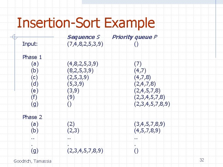
Insertion-Sort Example Input: Sequence S (7, 4, 8, 2, 5, 3, 9) Phase 1 (a) (b) (c) (d) (e) (f) (g) (4, 8, 2, 5, 3, 9) (2, 5, 3, 9) (3, 9) () (7) (4, 7, 8) (2, 4, 5, 7, 8) (2, 3, 4, 5, 7, 8, 9) Phase 2 (a) (b). . . (g) (2, 3). . . (2, 3, 4, 5, 7, 8, 9) (4, 5, 7, 8, 9). . . () Goodrich, Tamassia Priority queue P () 32

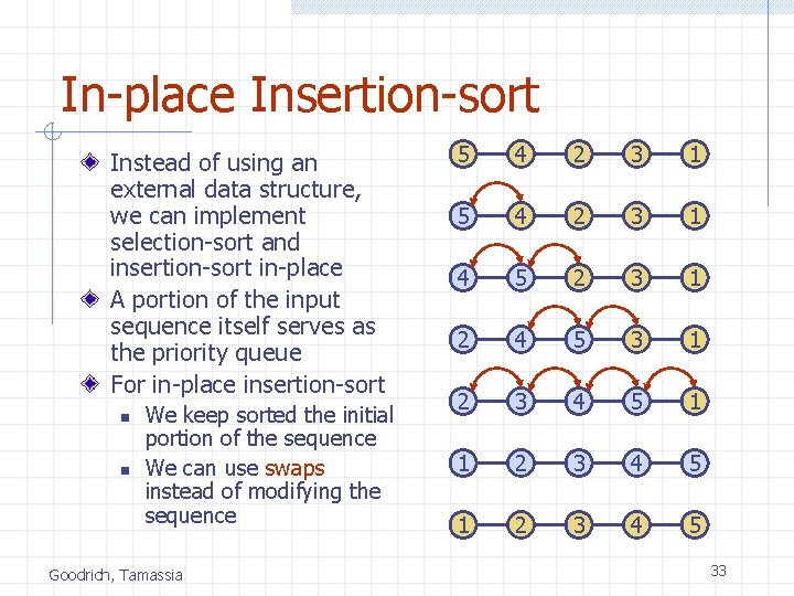
In-place Insertion-sort Instead of using an external data structure, we can implement selection-sort and insertion-sort in-place A portion of the input sequence itself serves as the priority queue For in-place insertion-sort n n We keep sorted the initial portion of the sequence We can use swaps instead of modifying the sequence Goodrich, Tamassia 5 4 2 3 1 4 5 2 3 1 2 4 5 3 1 2 3 4 5 33

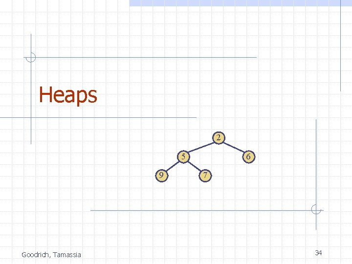
Heaps 2 5 9 Goodrich, Tamassia 6 7 34

Recall Priority Queue ADT (§ 7. 1. 3) A priority queue stores a collection of entries Each entry is a pair (key, value) Main methods of the Priority Queue ADT n n insert(k, x) inserts an entry with key k and value x remove. Min() removes and returns the entry with smallest key Goodrich, Tamassia Additional methods n n min() returns, but does not remove, an entry with smallest key size(), is. Empty() Applications: n n n Standby flyers Auctions Stock market 35

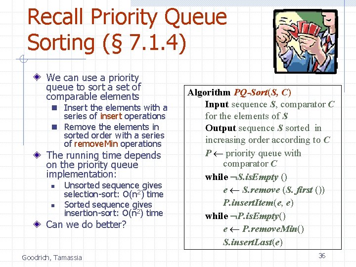
Recall Priority Queue Sorting (§ 7. 1. 4) We can use a priority queue to sort a set of comparable elements n Insert the elements with a series of insert operations n Remove the elements in sorted order with a series of remove. Min operations The running time depends on the priority queue implementation: n n Unsorted sequence gives selection-sort: O(n 2) time Sorted sequence gives insertion-sort: O(n 2) time Can we do better? Goodrich, Tamassia Algorithm PQ-Sort(S, C) Input sequence S, comparator C for the elements of S Output sequence S sorted in increasing order according to C P priority queue with comparator C while S. is. Empty () e S. remove (S. first ()) P. insert. Item(e, e) while P. is. Empty() e P. remove. Min() S. insert. Last(e) 36

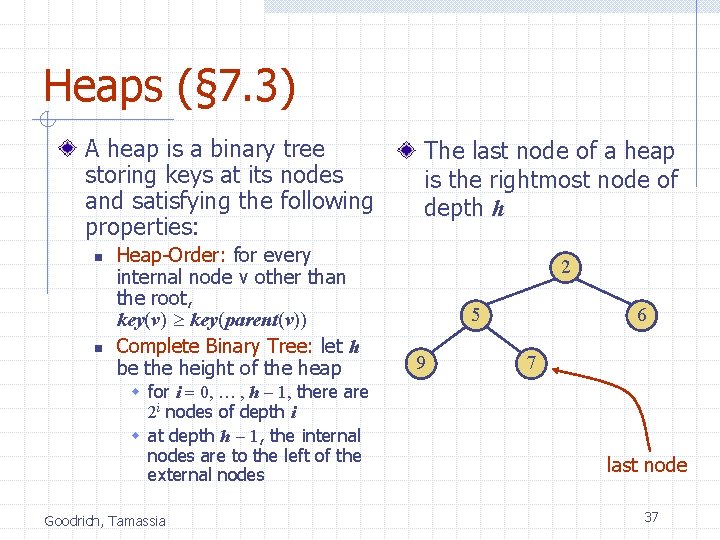
Heaps (§ 7. 3) A heap is a binary tree storing keys at its nodes and satisfying the following properties: n n Heap-Order: for every internal node v other than the root, key(v) key(parent(v)) Complete Binary Tree: let h be the height of the heap w for i = 0, … , h - 1, there are 2 i nodes of depth i w at depth h - 1, the internal nodes are to the left of the external nodes Goodrich, Tamassia The last node of a heap is the rightmost node of depth h 2 5 9 6 7 last node 37

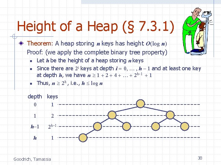
Height of a Heap (§ 7. 3. 1) Theorem: A heap storing n keys has height O(log n) Proof: (we apply the complete binary tree property) Let h be the height of a heap storing n keys Since there are 2 i keys at depth i = 0, … , h - 1 and at least one key at depth h, we have n 1 + 2 + 4 + … + 2 h-1 + 1 Thus, n 2 h , i. e. , h log n n depth keys 0 1 1 2 h-1 2 h-1 h 1 Goodrich, Tamassia 38

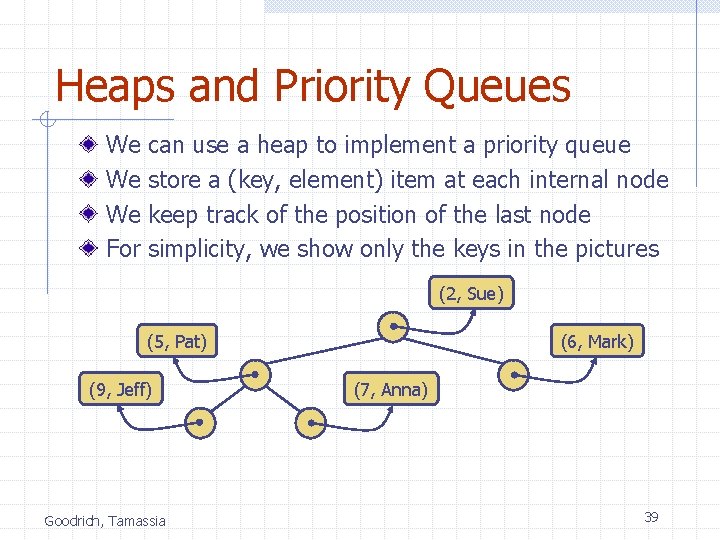
Heaps and Priority Queues We We We For can use a heap to implement a priority queue store a (key, element) item at each internal node keep track of the position of the last node simplicity, we show only the keys in the pictures (2, Sue) (5, Pat) (9, Jeff) Goodrich, Tamassia (6, Mark) (7, Anna) 39

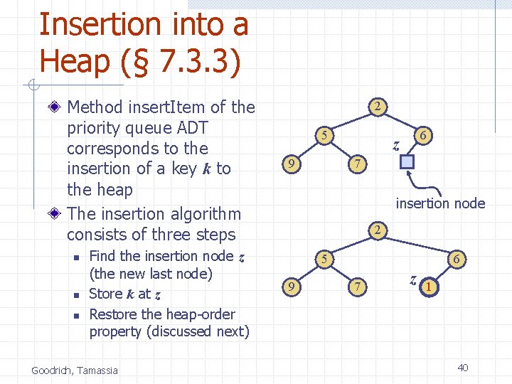
Insertion into a Heap (§ 7. 3. 3) Method insert. Item of the priority queue ADT corresponds to the insertion of a key k to the heap The insertion algorithm consists of three steps n n n Find the insertion node z (the new last node) Store k at z Restore the heap-order property (discussed next) Goodrich, Tamassia 2 5 9 6 z 7 insertion node 2 5 9 6 7 z 1 40

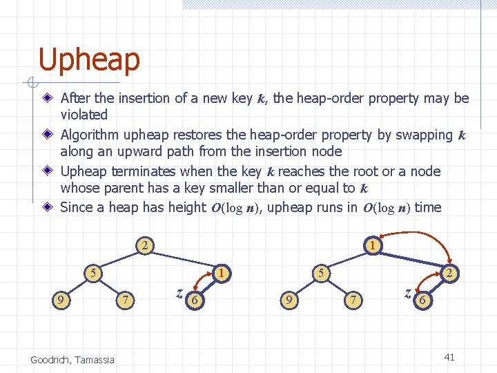
Upheap After the insertion of a new key k, the heap-order property may be violated Algorithm upheap restores the heap-order property by swapping k along an upward path from the insertion node Upheap terminates when the key k reaches the root or a node whose parent has a key smaller than or equal to k Since a heap has height O(log n), upheap runs in O(log n) time 2 1 5 9 Goodrich, Tamassia 1 7 z 6 5 9 2 7 z 6 41

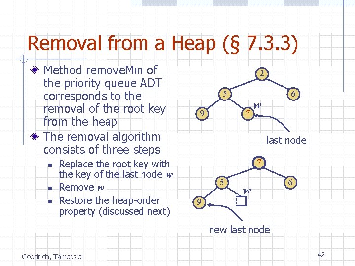
Removal from a Heap (§ 7. 3. 3) Method remove. Min of the priority queue ADT corresponds to the removal of the root key from the heap The removal algorithm consists of three steps n n n Replace the root key with the key of the last node w Remove w Restore the heap-order property (discussed next) 2 5 9 6 7 w last node 7 5 w 6 9 new last node Goodrich, Tamassia 42

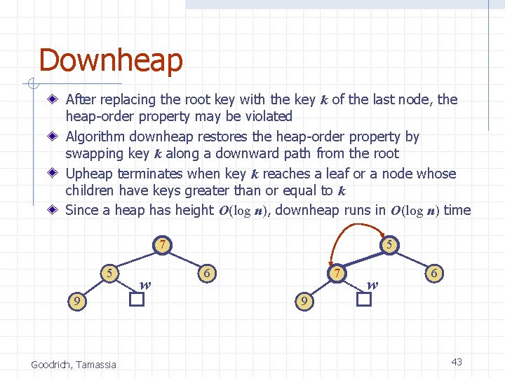
Downheap After replacing the root key with the key k of the last node, the heap-order property may be violated Algorithm downheap restores the heap-order property by swapping key k along a downward path from the root Upheap terminates when key k reaches a leaf or a node whose children have keys greater than or equal to k Since a heap has height O(log n), downheap runs in O(log n) time 7 5 9 Goodrich, Tamassia w 5 6 7 w 6 9 43

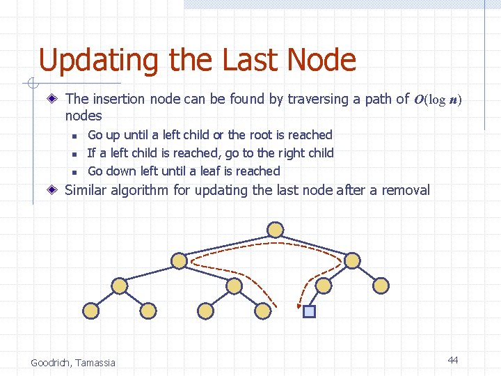
Updating the Last Node The insertion node can be found by traversing a path of O(log n) nodes n n n Go up until a left child or the root is reached If a left child is reached, go to the right child Go down left until a leaf is reached Similar algorithm for updating the last node after a removal Goodrich, Tamassia 44

Heap-Sort (§ 2. 4. 4) Consider a priority queue with n items implemented by means of a heap n n n the space used is O(n) methods insert and remove. Min take O(log n) time methods size, is. Empty, and min take time O(1) time Goodrich, Tamassia Using a heap-based priority queue, we can sort a sequence of n elements in O(n log n) time The resulting algorithm is called heap-sort Heap-sort is much faster than quadratic sorting algorithms, such as insertion-sort and selection-sort 45

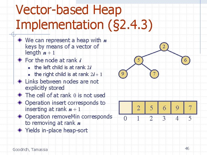
Vector-based Heap Implementation (§ 2. 4. 3) We can represent a heap with n keys by means of a vector of length n + 1 For the node at rank i n n the left child is at rank 2 i the right child is at rank 2 i + 1 Links between nodes are not explicitly stored The cell of at rank 0 is not used Operation insert corresponds to inserting at rank n + 1 Operation remove. Min corresponds to removing at rank n Yields in-place heap-sort Goodrich, Tamassia 2 5 6 9 0 7 2 5 6 9 7 1 2 3 4 5 46

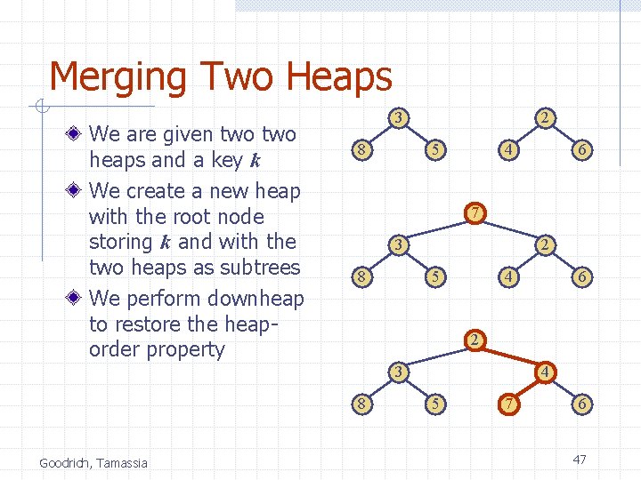
Merging Two Heaps We are given two heaps and a key k We create a new heap with the root node storing k and with the two heaps as subtrees We perform downheap to restore the heaporder property 3 8 2 5 4 7 3 8 2 5 4 6 2 3 8 Goodrich, Tamassia 6 4 5 7 6 47

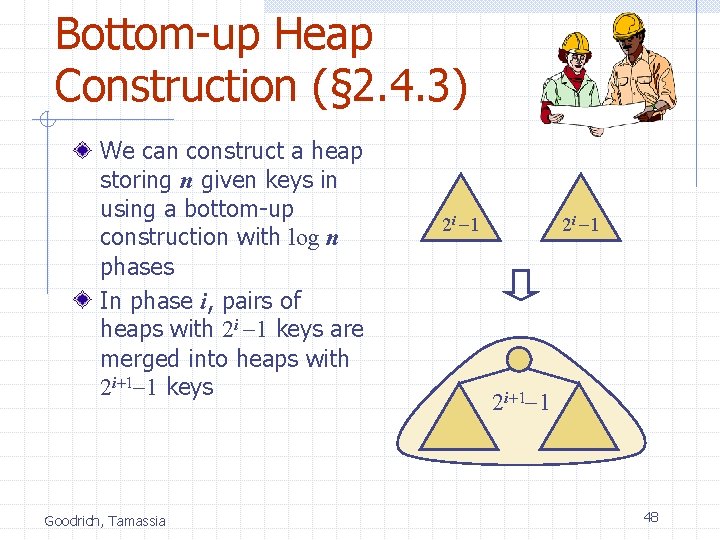
Bottom-up Heap Construction (§ 2. 4. 3) We can construct a heap storing n given keys in using a bottom-up construction with log n phases In phase i, pairs of heaps with 2 i -1 keys are merged into heaps with 2 i+1 -1 keys Goodrich, Tamassia 2 i -1 2 i+1 -1 48

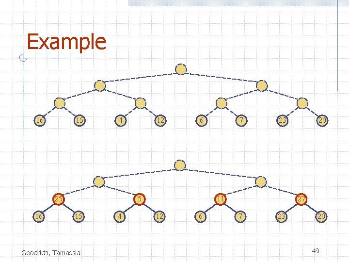
Example 16 15 4 25 16 12 6 5 15 Goodrich, Tamassia 4 7 23 11 12 6 20 27 7 23 20 49

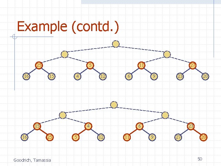
Example (contd. ) 25 16 5 15 4 15 16 11 12 6 4 25 Goodrich, Tamassia 5 27 9 23 6 12 11 20 23 9 27 20 50

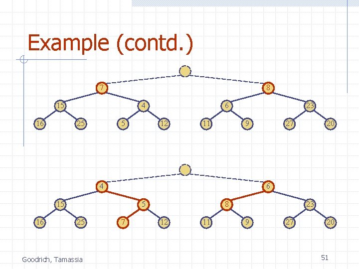
Example (contd. ) 7 8 15 16 4 25 5 6 12 11 23 9 4 5 25 Goodrich, Tamassia 20 6 15 16 27 7 8 12 11 23 9 27 20 51

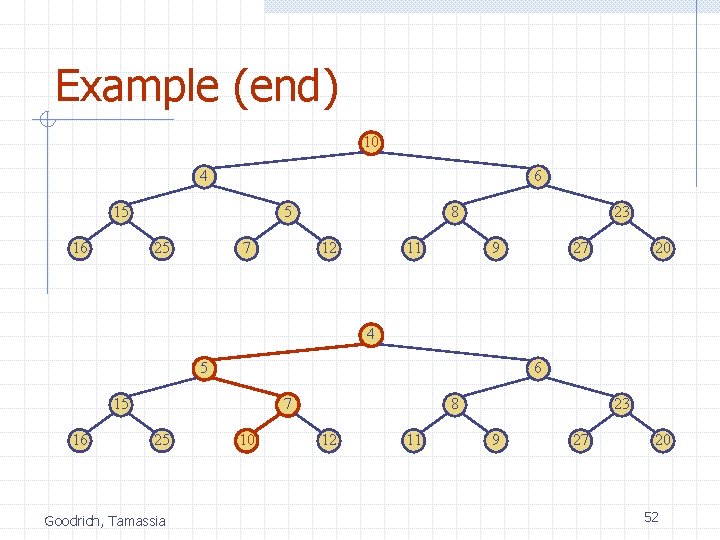
Example (end) 10 4 6 15 16 5 25 7 8 12 11 23 9 27 20 4 5 6 15 16 7 25 Goodrich, Tamassia 10 8 12 11 23 9 27 20 52

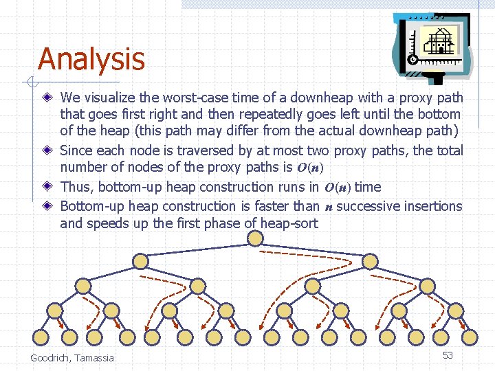
Analysis We visualize the worst-case time of a downheap with a proxy path that goes first right and then repeatedly goes left until the bottom of the heap (this path may differ from the actual downheap path) Since each node is traversed by at most two proxy paths, the total number of nodes of the proxy paths is O(n) Thus, bottom-up heap construction runs in O(n) time Bottom-up heap construction is faster than n successive insertions and speeds up the first phase of heap-sort Goodrich, Tamassia 53

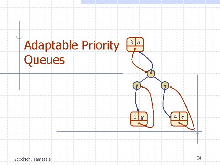
Adaptable Priority Queues 3 a 5 g Goodrich, Tamassia 4 e 54

Recall the Entry and Priority Queue ADTs (§ 7. 1) An entry stores a (key, value) pair within a data structure Methods of the entry ADT: n n key(): returns the key associated with this entry value(): returns the value paired with the key associated with this entry Goodrich, Tamassia Priority Queue ADT: n n insert(k, x) inserts an entry with key k and value x remove. Min() removes and returns the entry with smallest key min() returns, but does not remove, an entry with smallest key size(), is. Empty() 55

Motivating Example Suppose we have an online trading system where orders to purchase and sell a given stock are stored in two priority queues (one for sell orders and one for buy orders) as (p, s) entries: n n The key, p, of an order is the price The value, s, for an entry is the number of shares A buy order (p, s) is executed when a sell order (p’, s’) with price p’<p is added (the execution is complete if s’>s) A sell order (p, s) is executed when a buy order (p’, s’) with price p’>p is added (the execution is complete if s’>s) What if someone wishes to cancel their order before it executes? What if someone wishes to update the price or number of shares for their order? Goodrich, Tamassia 56

Methods of the Adaptable Priority Queue ADT (§ 7. 4) remove(e): Remove from P and return entry e. replace. Key(e, k): Replace with k and return the key of entry e of P; an error condition occurs if k is invalid (that is, k cannot becompared with other keys). replace. Value(e, x): Replace with x and return the value of entry e of P. Goodrich, Tamassia 57

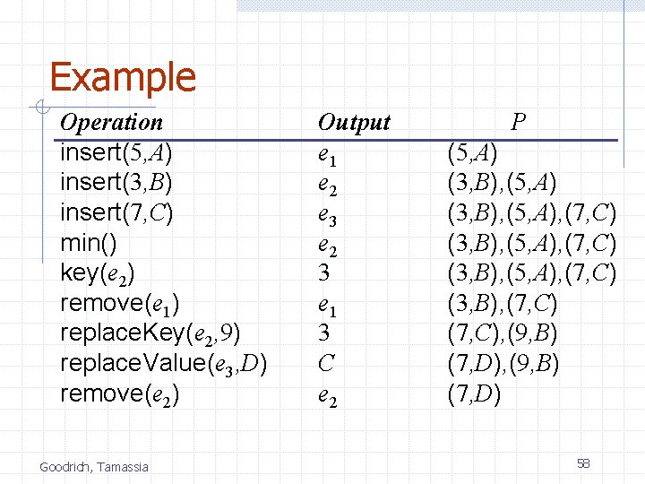
Example Operation insert(5, A) insert(3, B) insert(7, C) min() key(e 2) remove(e 1) replace. Key(e 2, 9) replace. Value(e 3, D) remove(e 2) Goodrich, Tamassia Output e 1 e 2 e 3 e 2 3 e 1 3 C e 2 P (5, A) (3, B), (5, A), (7, C) (3, B), (7, C), (9, B) (7, D) 58

Locating Entries In order to implement the operations remove(k), replace. Key(e), and replace. Value(k), we need fast ways of locating an entry e in a priority queue. We can always just search the entire data structure to find an entry e, but there are better ways for locating entries. Goodrich, Tamassia 59

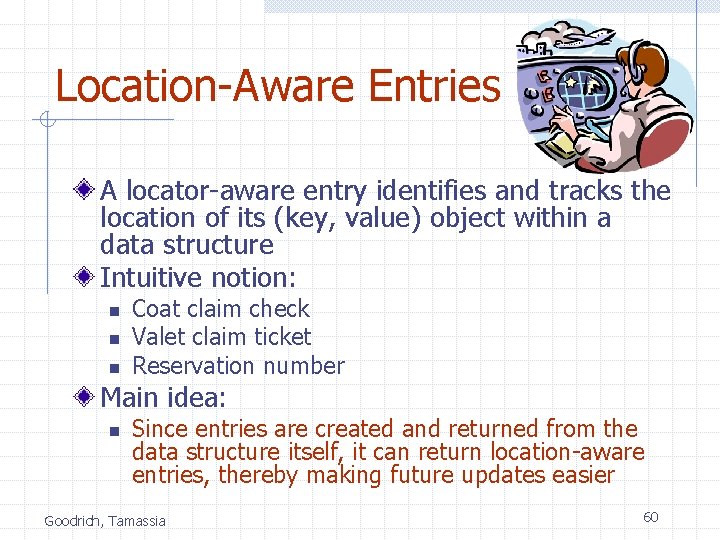
Location-Aware Entries A locator-aware entry identifies and tracks the location of its (key, value) object within a data structure Intuitive notion: n n n Coat claim check Valet claim ticket Reservation number Main idea: n Since entries are created and returned from the data structure itself, it can return location-aware entries, thereby making future updates easier Goodrich, Tamassia 60

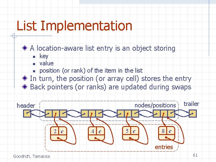
List Implementation A location-aware list entry is an object storing n n n key value position (or rank) of the item in the list In turn, the position (or array cell) stores the entry Back pointers (or ranks) are updated during swaps nodes/positions header 2 c 4 c 5 c trailer 8 c entries Goodrich, Tamassia 61

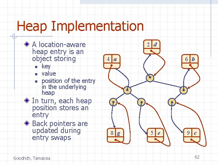
Heap Implementation A location-aware heap entry is an object storing n n n key value position of the entry in the underlying heap In turn, each heap position stores an entry Back pointers are updated during entry swaps Goodrich, Tamassia 2 d 4 a 8 g 6 b 5 e 9 c 62

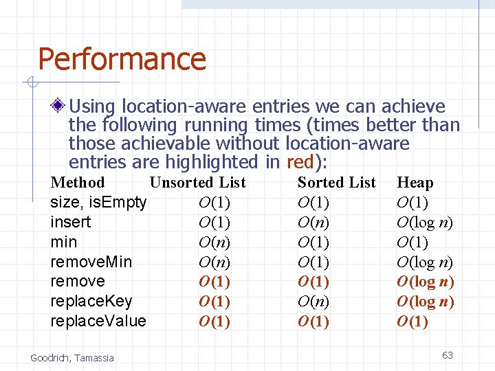
Performance Using location-aware entries we can achieve the following running times (times better than those achievable without location-aware entries are highlighted in red): Method Unsorted List size, is. Empty O(1) insert O(1) min O(n) remove. Min O(n) remove O(1) replace. Key O(1) replace. Value O(1) Goodrich, Tamassia Sorted List O(1) O(n) O(1) Heap O(1) O(log n) O(1) 63

Maps Goodrich, Tamassia 64

Maps A map models a searchable collection of key-value entries The main operations of a map are for searching, inserting, and deleting items Multiple entries with the same key are not allowed Applications: n n address book student-record database Goodrich, Tamassia 65

The Map ADT (§ 8. 1) Map ADT methods: n n n get(k): if the map M has an entry with key k, return its assoiciated value; else, return null put(k, v): insert entry (k, v) into the map M; if key k is not already in M, then return null; else, return old value associated with k remove(k): if the map M has an entry with key k, remove it from M and return its associated value; else, return null size(), is. Empty() keys(): return an iterator of the keys in M values(): return an iterator of the values in M Goodrich, Tamassia 66

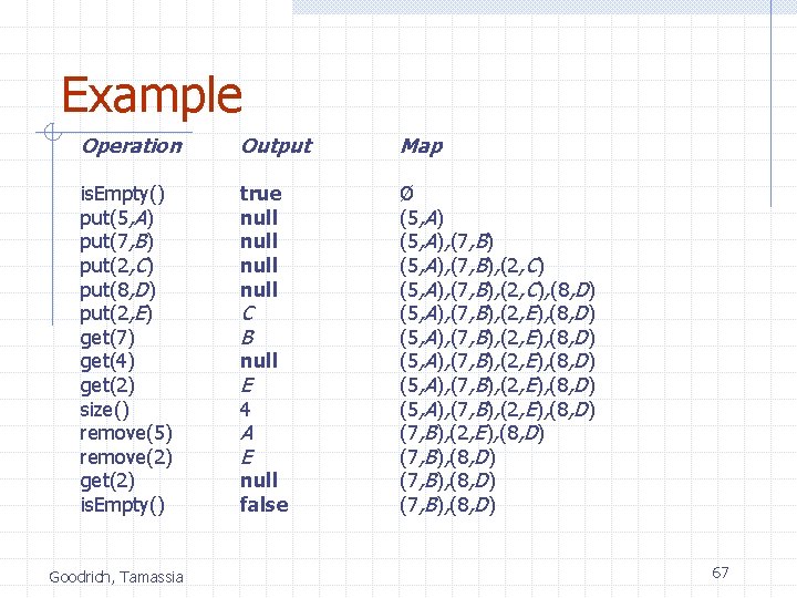
Example Operation Output Map is. Empty() put(5, A) put(7, B) put(2, C) put(8, D) put(2, E) get(7) get(4) get(2) size() remove(5) remove(2) get(2) is. Empty() true null Ø (5, A), (7, B), (2, C), (8, D) (5, A), (7, B), (2, E), (8, D) (5, A), (7, B), (2, E), (8, D) (7, B), (8, D) Goodrich, Tamassia C B null E 4 A E null false 67

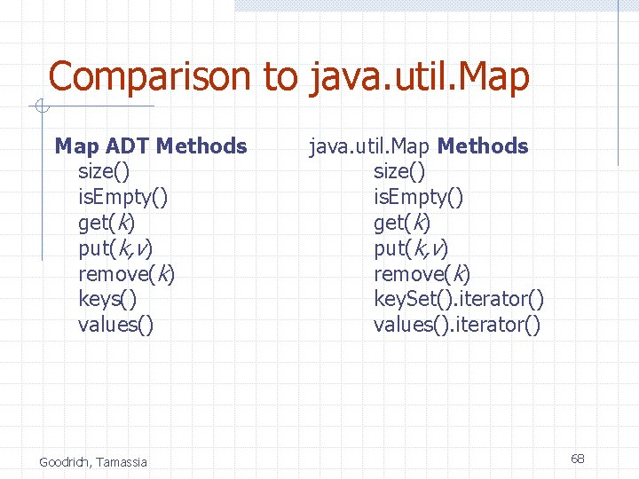
Comparison to java. util. Map ADT Methods size() is. Empty() get(k) put(k, v) remove(k) keys() values() Goodrich, Tamassia java. util. Map Methods size() is. Empty() get(k) put(k, v) remove(k) key. Set(). iterator() values(). iterator() 68

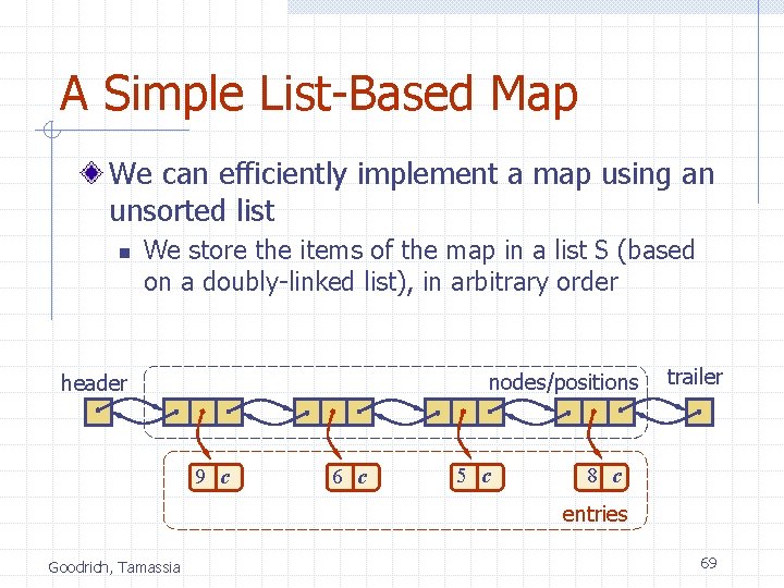
A Simple List-Based Map We can efficiently implement a map using an unsorted list n We store the items of the map in a list S (based on a doubly-linked list), in arbitrary order nodes/positions header 9 c 6 c 5 c trailer 8 c entries Goodrich, Tamassia 69

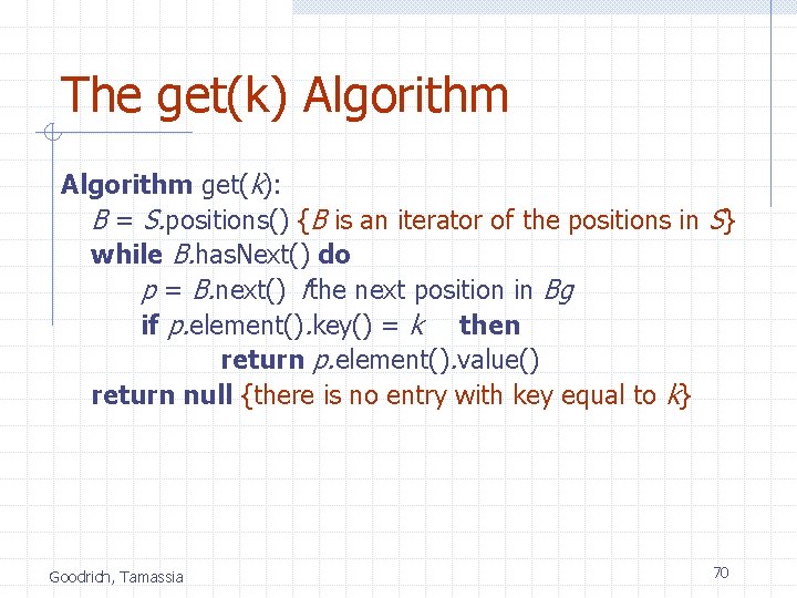
The get(k) Algorithm get(k): B = S. positions() {B is an iterator of the positions in S} while B. has. Next() do p = B. next() fthe next position in Bg if p. element(). key() = k then return p. element(). value() return null {there is no entry with key equal to k} Goodrich, Tamassia 70

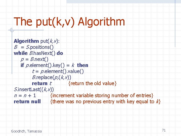
The put(k, v) Algorithm put(k, v): B = S. positions() while B. has. Next() do p = B. next() if p. element(). key() = k then t = p. element(). value() B. replace(p, (k, v)) return t {return the old value} S. insert. Last((k, v)) n=n+1 {increment variable storing number of entries} return null {there was no previous entry with key equal to k} Goodrich, Tamassia 71

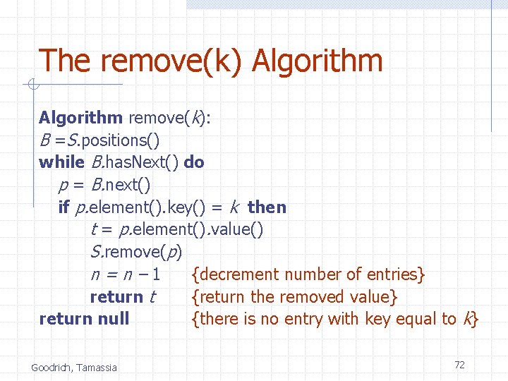
The remove(k) Algorithm remove(k): B =S. positions() while B. has. Next() do p = B. next() if p. element(). key() = k then t = p. element(). value() S. remove(p) n=n– 1 {decrement number of entries} return t {return the removed value} return null {there is no entry with key equal to k} Goodrich, Tamassia 72

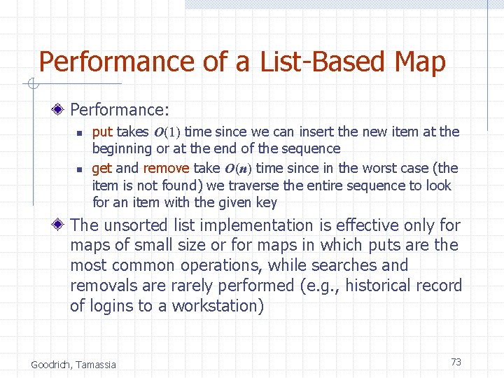
Performance of a List-Based Map Performance: n n put takes O(1) time since we can insert the new item at the beginning or at the end of the sequence get and remove take O(n) time since in the worst case (the item is not found) we traverse the entire sequence to look for an item with the given key The unsorted list implementation is effective only for maps of small size or for maps in which puts are the most common operations, while searches and removals are rarely performed (e. g. , historical record of logins to a workstation) Goodrich, Tamassia 73

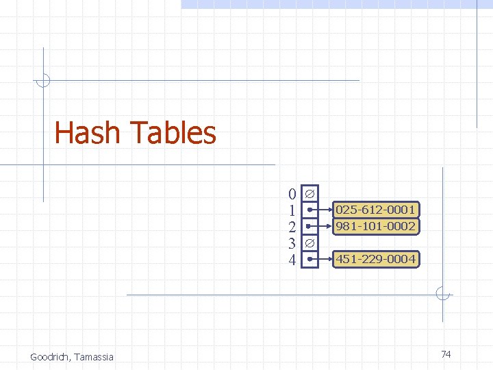
Hash Tables 0 1 2 3 4 Goodrich, Tamassia 025 -612 -0001 981 -101 -0002 451 -229 -0004 74

Recall the Map ADT (§ 8. 1) Map ADT methods: n n n get(k): if the map M has an entry with key k, return its assoiciated value; else, return null put(k, v): insert entry (k, v) into the map M; if key k is not already in M, then return null; else, return old value associated with k remove(k): if the map M has an entry with key k, remove it from M and return its associated value; else, return null size(), is. Empty() keys(): return an iterator of the keys in M values(): return an iterator of the values in M Goodrich, Tamassia 75

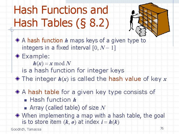
Hash Functions and Hash Tables (§ 8. 2) A hash function h maps keys of a given type to integers in a fixed interval [0, N - 1] Example: h(x) = x mod N is a hash function for integer keys The integer h(x) is called the hash value of key x A hash table for a given key type consists of n Hash function h n Array (called table) of size N When implementing a map with a hash table, the goal is to store item (k, o) at index i = h(k) Goodrich, Tamassia 76

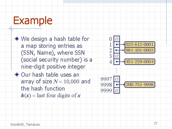
Example Goodrich, Tamassia 0 1 2 3 4 025 -612 -0001 981 -101 -0002 451 -229 -0004 … We design a hash table for a map storing entries as (SSN, Name), where SSN (social security number) is a nine-digit positive integer Our hash table uses an array of size N = 10, 000 and the hash function h(x) = last four digits of x 9997 9998 9999 200 -751 -9998 77

Hash Functions (§ 8. 2. 2) A hash function is usually specified as the composition of two functions: Hash code: h 1: keys integers Compression function: h 2: integers [0, N - 1] Goodrich, Tamassia The hash code is applied first, and the compression function is applied next on the result, i. e. , h(x) = h 2(h 1(x)) The goal of the hash function is to “disperse” the keys in an apparently random way 78

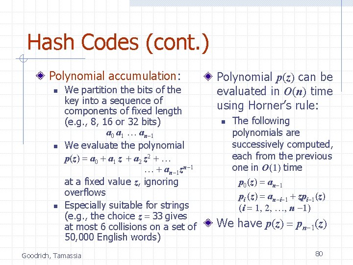
Hash Codes (§ 8. 2. 3) Memory address: n n We reinterpret the memory address of the key object as an integer (default hash code of all Java objects) Good in general, except for numeric and string keys Integer cast: n n We reinterpret the bits of the key as an integer Suitable for keys of length less than or equal to the number of bits of the integer type (e. g. , byte, short, int and float in Java) Goodrich, Tamassia Component sum: n n We partition the bits of the key into components of fixed length (e. g. , 16 or 32 bits) and we sum the components (ignoring overflows) Suitable for numeric keys of fixed length greater than or equal to the number of bits of the integer type (e. g. , long and double in Java) 79

Hash Codes (cont. ) Polynomial accumulation: n n n We partition the bits of the key into a sequence of components of fixed length (e. g. , 8, 16 or 32 bits) a 0 a 1 … an-1 We evaluate the polynomial p(z) = a 0 + a 1 z + a 2 z 2 + … … + an-1 zn-1 at a fixed value z, ignoring overflows Especially suitable for strings (e. g. , the choice z = 33 gives at most 6 collisions on a set of 50, 000 English words) Goodrich, Tamassia Polynomial p(z) can be evaluated in O(n) time using Horner’s rule: n The following polynomials are successively computed, each from the previous one in O(1) time p 0(z) = an-1 pi (z) = an-i-1 + zpi-1(z) (i = 1, 2, …, n -1) We have p(z) = pn-1(z) 80

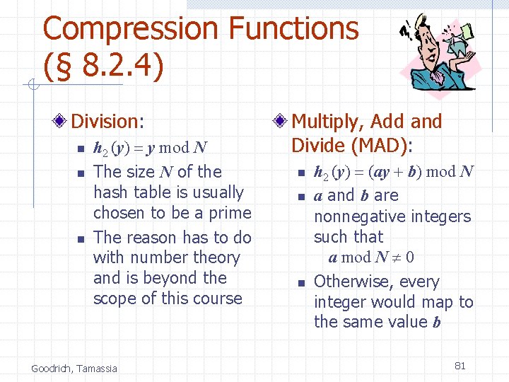
Compression Functions (§ 8. 2. 4) Division: n n n h 2 (y) = y mod N The size N of the hash table is usually chosen to be a prime The reason has to do with number theory and is beyond the scope of this course Goodrich, Tamassia Multiply, Add and Divide (MAD): n n n h 2 (y) = (ay + b) mod N a and b are nonnegative integers such that a mod N 0 Otherwise, every integer would map to the same value b 81

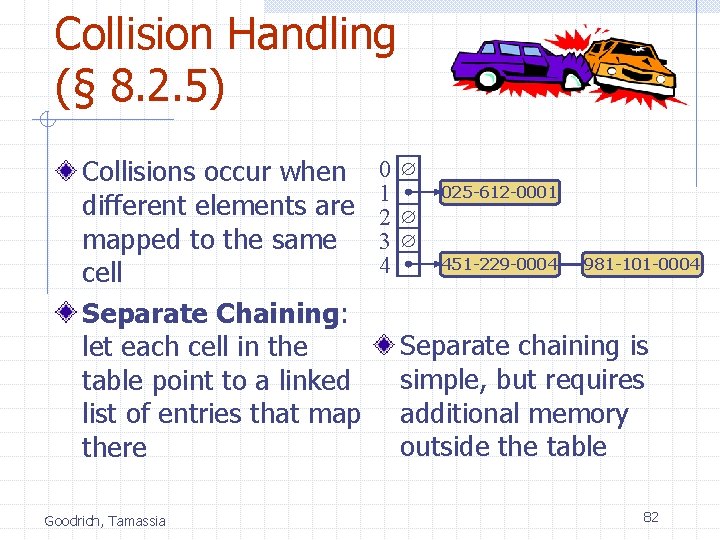
Collision Handling (§ 8. 2. 5) Collisions occur when different elements are mapped to the same cell Separate Chaining: let each cell in the table point to a linked list of entries that map there Goodrich, Tamassia 0 1 2 3 4 025 -612 -0001 451 -229 -0004 981 -101 -0004 Separate chaining is simple, but requires additional memory outside the table 82

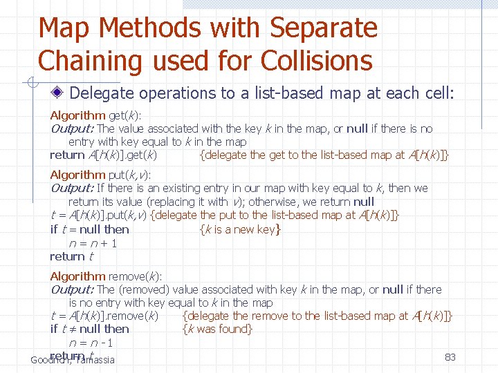
Map Methods with Separate Chaining used for Collisions Delegate operations to a list-based map at each cell: Algorithm get(k): Output: The value associated with the key k in the map, or null if there is no entry with key equal to k in the map return A[h(k)]. get(k) {delegate the get to the list-based map at A[h(k)]} Algorithm put(k, v): Output: If there is an existing entry in our map with key equal to k, then we return its value (replacing it with v); otherwise, we return null t = A[h(k)]. put(k, v) {delegate the put to the list-based map at A[h(k)]} if t = null then {k is a new key} n=n+1 return t Algorithm remove(k): Output: The (removed) value associated with key k in the map, or null if there is no entry with key equal to k in the map t = A[h(k)]. remove(k) {delegate the remove to the list-based map at A[h(k)]} if t ≠ null then {k was found} n=n-1 return t 83 Goodrich, Tamassia

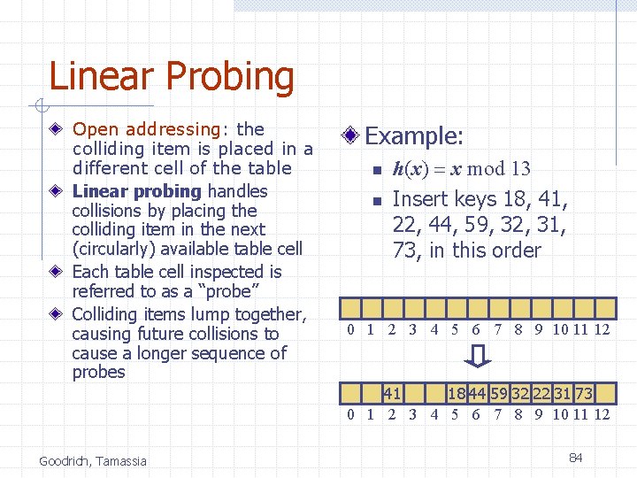
Linear Probing Open addressing: the colliding item is placed in a different cell of the table Linear probing handles collisions by placing the colliding item in the next (circularly) available table cell Each table cell inspected is referred to as a “probe” Colliding items lump together, causing future collisions to cause a longer sequence of probes Example: n n h(x) = x mod 13 Insert keys 18, 41, 22, 44, 59, 32, 31, 73, in this order 0 1 2 3 4 5 6 7 8 9 10 11 12 41 18 44 59 32 22 31 73 0 1 2 3 4 5 6 7 8 9 10 11 12 Goodrich, Tamassia 84

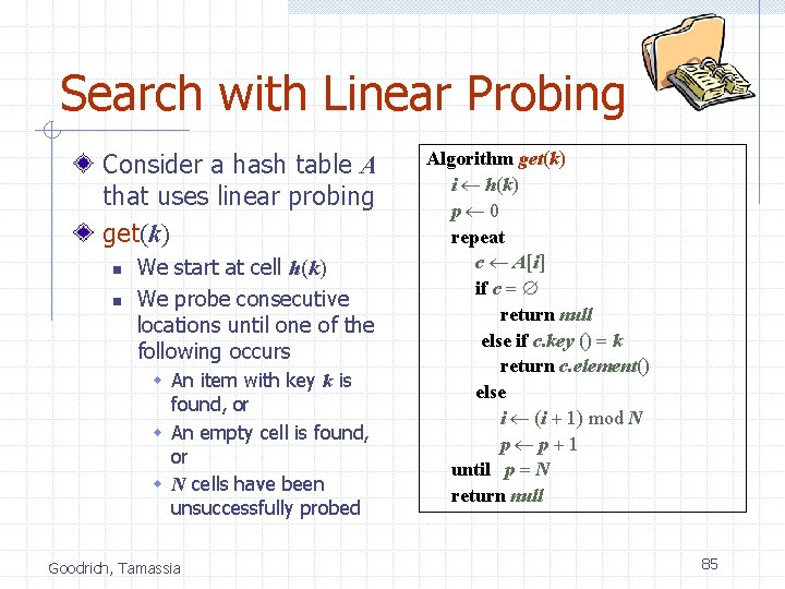
Search with Linear Probing Consider a hash table A that uses linear probing get(k) n n We start at cell h(k) We probe consecutive locations until one of the following occurs w An item with key k is found, or w An empty cell is found, or w N cells have been unsuccessfully probed Goodrich, Tamassia Algorithm get(k) i h(k) p 0 repeat c A[i] if c = return null else if c. key () = k return c. element() else i (i + 1) mod N p p+1 until p = N return null 85

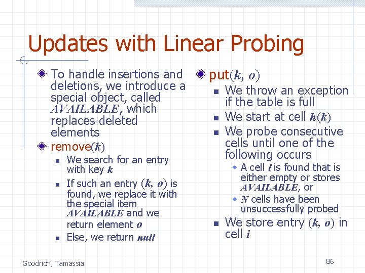
Updates with Linear Probing To handle insertions and deletions, we introduce a special object, called AVAILABLE, which replaces deleted elements remove(k) n n n We search for an entry with key k If such an entry (k, o) is found, we replace it with the special item AVAILABLE and we return element o Else, we return null Goodrich, Tamassia put(k, o) n n n We throw an exception if the table is full We start at cell h(k) We probe consecutive cells until one of the following occurs w A cell i is found that is either empty or stores AVAILABLE, or w N cells have been unsuccessfully probed n We store entry (k, o) in cell i 86

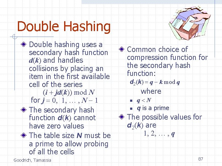
Double Hashing Double hashing uses a secondary hash function d(k) and handles collisions by placing an item in the first available cell of the series (i + jd(k)) mod N for j = 0, 1, … , N - 1 The secondary hash function d(k) cannot have zero values The table size N must be a prime to allow probing of all the cells Goodrich, Tamassia Common choice of compression function for the secondary hash function: d 2(k) = q - k mod q where n n q<N q is a prime The possible values for d 2(k) are 1, 2, … , q 87

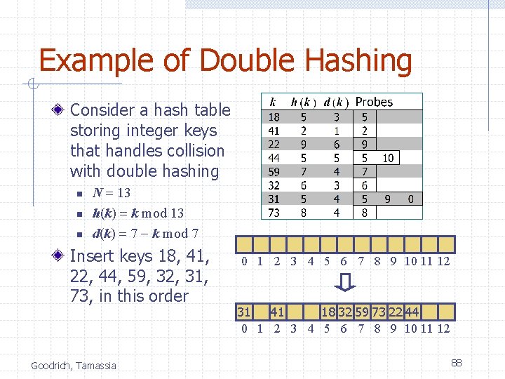
Example of Double Hashing Consider a hash table storing integer keys that handles collision with double hashing n n n N = 13 h(k) = k mod 13 d(k) = 7 - k mod 7 Insert keys 18, 41, 22, 44, 59, 32, 31, 73, in this order Goodrich, Tamassia 0 1 2 3 4 5 6 7 8 9 10 11 12 31 41 18 32 59 73 22 44 0 1 2 3 4 5 6 7 8 9 10 11 12 88

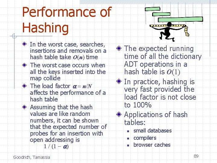
Performance of Hashing In the worst case, searches, insertions and removals on a hash table take O(n) time The worst case occurs when all the keys inserted into the map collide The load factor a = n/N affects the performance of a hash table Assuming that the hash values are like random numbers, it can be shown that the expected number of probes for an insertion with open addressing is 1 / (1 - a) Goodrich, Tamassia The expected running time of all the dictionary ADT operations in a hash table is O(1) In practice, hashing is very fast provided the load factor is not close to 100% Applications of hash tables: n n n small databases compilers browser caches 89

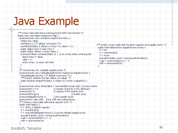
Java Example /** A hash table with linear probing and the MAD hash function */ public class Hash. Table implements Map { protected static class Hash. Entry implements Entry { Object key, value; Hash. Entry () { /* default constructor */ } /** Creates a hash table with the given capacity and equality tester. */ Hash. Entry(Object k, Object v) { key = k; value = v; } public Hash. Table(int b. N, Equality. Tester tester) { public Object key() { return key; } N = b. N; public Object value() { return value; } A = new Entry[N]; protected Object set. Value(Object v) { // set a new value, returning old T = tester; Object temp = value; java. util. Random rand = new java. util. Random(); value = v; scale = rand. next. Int(N-1) + 1; return temp; // return old value shift = rand. next. Int(N); } } } /** Nested class for a default equality tester */ protected static class Default. Equality. Tester implements Equality. Tester { Default. Equality. Tester() { /* default constructor */ } /** Returns whether the two objects are equal. */ public boolean is. Equal. To(Object a, Object b) { return a. equals(b); } } protected static Entry AVAILABLE = new Hash. Entry(null, null); // empty marker protected int n = 0; // number of entries in the dictionary protected int N; // capacity of the bucket array protected Entry[] A; // bucket array protected Equality. Tester T; // the equality tester protected int scale, shift; // the shift and scaling factors /** Creates a hash table with initial capacity 1023. */ public Hash. Table() { N = 1023; // default capacity A = new Entry[N]; T = new Default. Equality. Tester(); // use the default equality tester java. util. Random rand = new java. util. Random(); scale = rand. next. Int(N-1) + 1; shift = rand. next. Int(N); } Goodrich, Tamassia 90

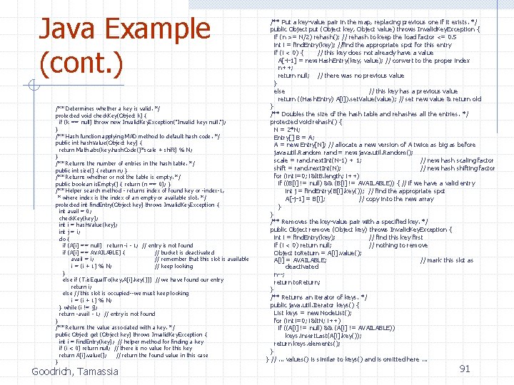
Java Example (cont. ) /** Determines whether a key is valid. */ protected void check. Key(Object k) { if (k == null) throw new Invalid. Key. Exception("Invalid key: null. "); } /** Hash function applying MAD method to default hash code. */ public int hash. Value(Object key) { return Math. abs(key. hash. Code()*scale + shift) % N; } /** Returns the number of entries in the hash table. */ public int size() { return n; } /** Returns whether or not the table is empty. */ public boolean is. Empty() { return (n == 0); } /** Helper search method - returns index of found key or -index-1, * where index is the index of an empty or available slot. */ protected int find. Entry(Object key) throws Invalid. Key. Exception { int avail = 0; check. Key(key); int i = hash. Value(key); int j = i; do { if (A[i] == null) return -i - 1; // entry is not found if (A[i] == AVAILABLE) { // bucket is deactivated avail = i; // remember that this slot is available i = (i + 1) % N; // keep looking } else if (T. is. Equal. To(key, A[i]. key())) // we have found our entry return i; else // this slot is occupied--we must keep looking i = (i + 1) % N; } while (i != j); return -avail - 1; // entry is not found } /** Returns the value associated with a key. */ public Object get (Object key) throws Invalid. Key. Exception { int i = find. Entry(key); // helper method for finding a key if (i < 0) return null; // there is no value for this key return A[i]. value(); // return the found value in this case } Goodrich, Tamassia /** Put a key-value pair in the map, replacing previous one if it exists. */ public Object put (Object key, Object value) throws Invalid. Key. Exception { if (n >= N/2) rehash(); // rehash to keep the load factor <= 0. 5 int i = find. Entry(key); //find the appropriate spot for this entry if (i < 0) { // this key does not already have a value A[-i-1] = new Hash. Entry(key, value); // convert to the proper index n++; return null; // there was no previous value } else // this key has a previous value return ((Hash. Entry) A[i]). set. Value(value); // set new value & return old } /** Doubles the size of the hash table and rehashes all the entries. */ protected void rehash() { N = 2*N; Entry[] B = A; A = new Entry[N]; // allocate a new version of A twice as big as before java. util. Random rand = new java. util. Random(); scale = rand. next. Int(N-1) + 1; // new hash scaling factor shift = rand. next. Int(N); // new hash shifting factor for (int i=0; i&lt. B. length; i++) if ((B[i] != null) && (B[i] != AVAILABLE)) { // if we have a valid entry int j = find. Entry(B[i]. key()); // find the appropriate spot A[-j-1] = B[i]; // copy into the new array } } /** Removes the key-value pair with a specified key. */ public Object remove (Object key) throws Invalid. Key. Exception { int i = find. Entry(key); // find this key first if (i < 0) return null; // nothing to remove Object to. Return = A[i]. value(); A[i] = AVAILABLE; // mark this slot as deactivated n--; return to. Return; } /** Returns an iterator of keys. */ public java. util. Iterator keys() { List keys = new Node. List(); for (int i=0; i&lt. N; i++) if ((A[i] != null) && (A[i] != AVAILABLE)) keys. insert. Last(A[i]. key()); return keys. elements(); } } //. . . values() is similar to keys() and is omitted here. . . 91

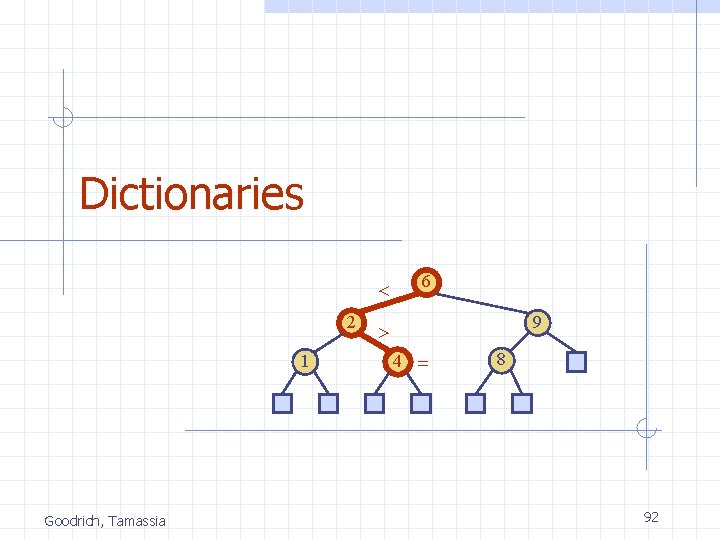
Dictionaries < 2 1 Goodrich, Tamassia 6 9 > 4 = 8 92

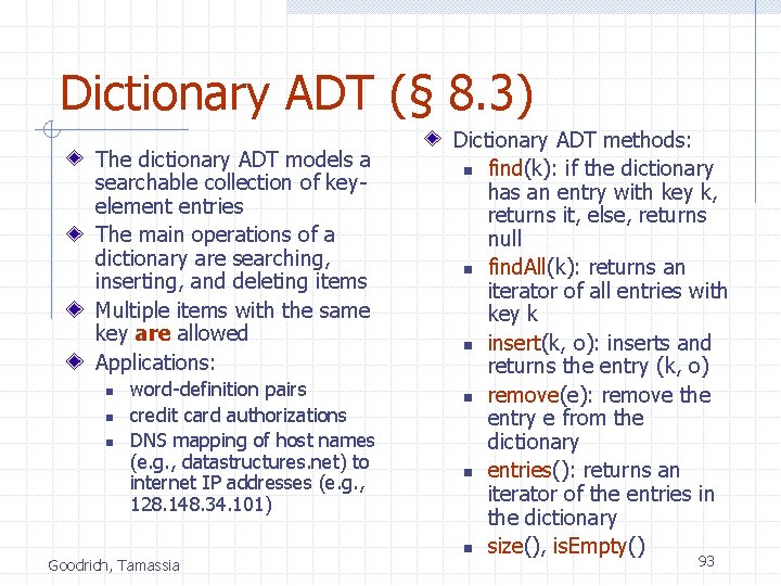
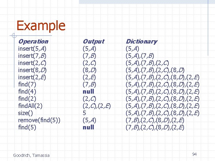
Dictionary ADT (§ 8. 3) The dictionary ADT models a searchable collection of keyelement entries The main operations of a dictionary are searching, inserting, and deleting items Multiple items with the same key are allowed Applications: n n n word-definition pairs credit card authorizations DNS mapping of host names (e. g. , datastructures. net) to internet IP addresses (e. g. , 128. 148. 34. 101) Goodrich, Tamassia Dictionary ADT methods: n find(k): if the dictionary has an entry with key k, returns it, else, returns null n find. All(k): returns an iterator of all entries with key k n insert(k, o): inserts and returns the entry (k, o) n remove(e): remove the entry e from the dictionary n entries(): returns an iterator of the entries in the dictionary n size(), is. Empty() 93

Example Operation insert(5, A) insert(7, B) insert(2, C) insert(8, D) insert(2, E) find(7) find(4) find(2) find. All(2) size() remove(find(5)) find(5) Goodrich, Tamassia Output (5, A) (7, B) (2, C) (8, D) (2, E) (7, B) null (2, C), (2, E) 5 (5, A) null Dictionary (5, A), (7, B), (2, C), (8, D) (5, A), (7, B), (2, C), (8, D), (2, E) (5, A), (7, B), (2, C), (8, D), (2, E) 94

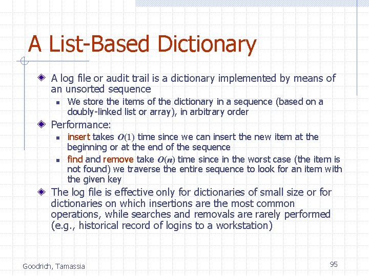
A List-Based Dictionary A log file or audit trail is a dictionary implemented by means of an unsorted sequence n We store the items of the dictionary in a sequence (based on a doubly-linked list or array), in arbitrary order Performance: n n insert takes O(1) time since we can insert the new item at the beginning or at the end of the sequence find and remove take O(n) time since in the worst case (the item is not found) we traverse the entire sequence to look for an item with the given key The log file is effective only for dictionaries of small size or for dictionaries on which insertions are the most common operations, while searches and removals are rarely performed (e. g. , historical record of logins to a workstation) Goodrich, Tamassia 95

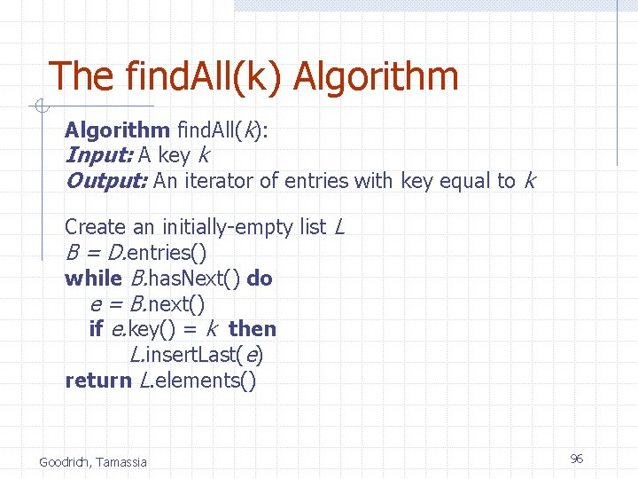
The find. All(k) Algorithm find. All(k): Input: A key k Output: An iterator of entries with key equal to k Create an initially-empty list L B = D. entries() while B. has. Next() do e = B. next() if e. key() = k then L. insert. Last(e) return L. elements() Goodrich, Tamassia 96

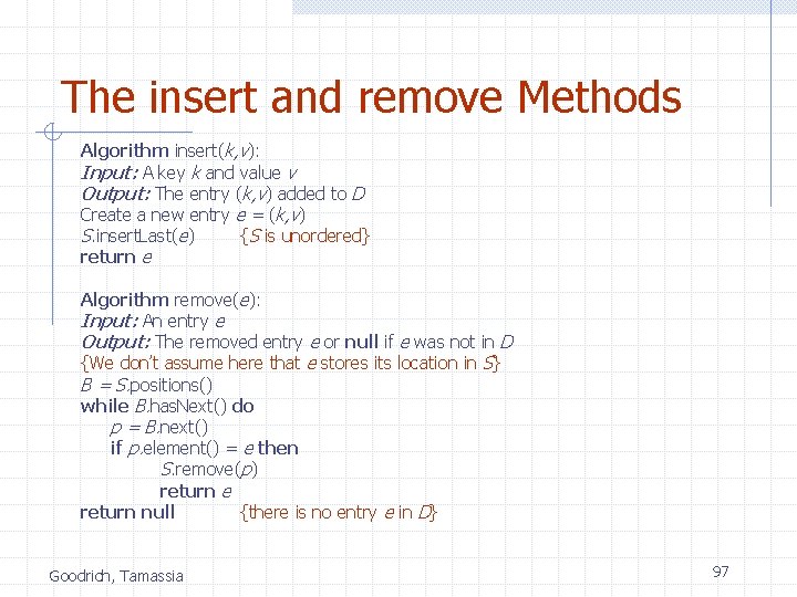
The insert and remove Methods Algorithm insert(k, v): Input: A key k and value v Output: The entry (k, v) added to D Create a new entry e = (k, v) S. insert. Last(e) {S is unordered} return e Algorithm remove(e): Input: An entry e Output: The removed entry e or null if e was not in D {We don’t assume here that e stores its location in S} B = S. positions() while B. has. Next() do p = B. next() if p. element() = e then S. remove(p) return e return null {there is no entry e in D} Goodrich, Tamassia 97

Hash Table Implementation We can also create a hash-table dictionary implementation. If we use separate chaining to handle collisions, then each operation can be delegated to a list-based dictionary stored at each hash table cell. Goodrich, Tamassia 98

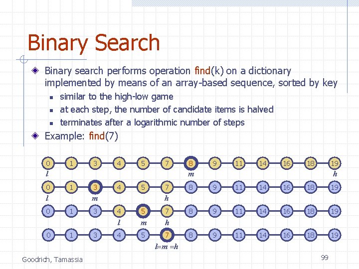
Binary Search Binary search performs operation find(k) on a dictionary implemented by means of an array-based sequence, sorted by key n n n similar to the high-low game at each step, the number of candidate items is halved terminates after a logarithmic number of steps Example: find(7) 0 1 3 4 5 7 1 0 3 4 5 m l 0 9 11 14 16 18 19 m l 0 8 1 1 3 3 7 h 8 9 11 14 16 18 19 h 4 5 7 l m h 4 5 7 l=m =h Goodrich, Tamassia 99

Search Table A search table is a dictionary implemented by means of a sorted array n n We store the items of the dictionary in an array-based sequence, sorted by key We use an external comparator for the keys Performance: n n n find takes O(log n) time, using binary search insert takes O(n) time since in the worst case we have to shift n/2 items to make room for the new item remove takes O(n) time since in the worst case we have to shift n/2 items to compact the items after the removal A search table is effective only for dictionaries of small size or for dictionaries on which searches are the most common operations, while insertions and removals are rarely performed (e. g. , credit card authorizations) Goodrich, Tamassia 100

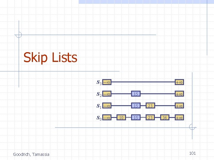
Skip Lists S 3 - S 2 - 15 S 1 - 15 23 S 0 - Goodrich, Tamassia + 10 + + 36 + 101

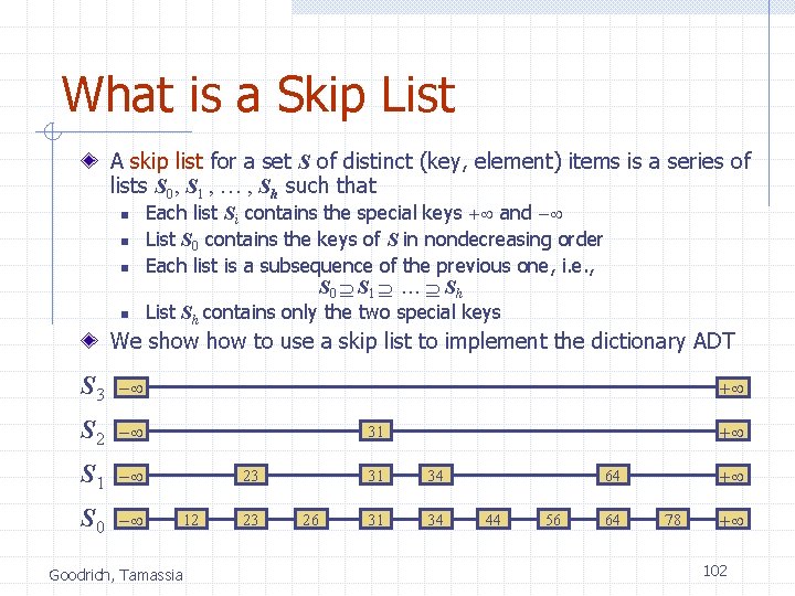
What is a Skip List A skip list for a set S of distinct (key, element) items is a series of lists S 0, S 1 , … , Sh such that n n Each list Si contains the special keys + and - List S 0 contains the keys of S in nondecreasing order Each list is a subsequence of the previous one, i. e. , S 0 S 1 … Sh List Sh contains only the two special keys We show to use a skip list to implement the dictionary ADT S 3 - S 2 - S 1 - S 0 - + + 31 23 12 Goodrich, Tamassia 23 26 31 34 + 64 44 56 64 78 + 102

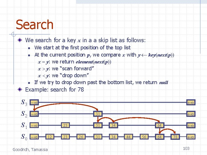
Search We search for a key x in a a skip list as follows: n n n We start at the first position of the top list At the current position p, we compare x with y key(next(p)) x = y: we return element(next(p)) x > y: we “scan forward” x < y: we “drop down” If we try to drop down past the bottom list, we return null Example: search for 78 S 3 - S 2 - S 1 - S 0 - + + 31 23 12 Goodrich, Tamassia 23 26 31 34 + 64 44 56 64 78 + 103

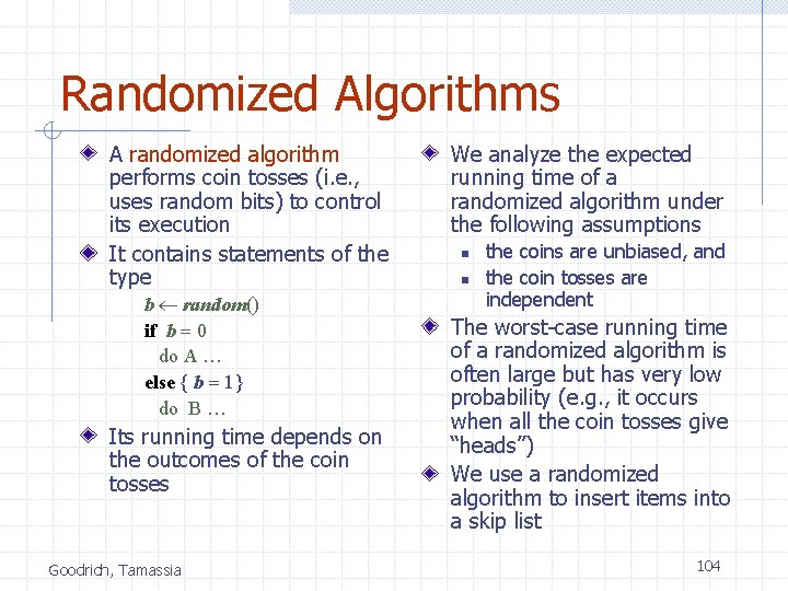
Randomized Algorithms A randomized algorithm performs coin tosses (i. e. , uses random bits) to control its execution It contains statements of the type b random() if b = 0 do A … else { b = 1} do B … Its running time depends on the outcomes of the coin tosses Goodrich, Tamassia We analyze the expected running time of a randomized algorithm under the following assumptions n n the coins are unbiased, and the coin tosses are independent The worst-case running time of a randomized algorithm is often large but has very low probability (e. g. , it occurs when all the coin tosses give “heads”) We use a randomized algorithm to insert items into a skip list 104

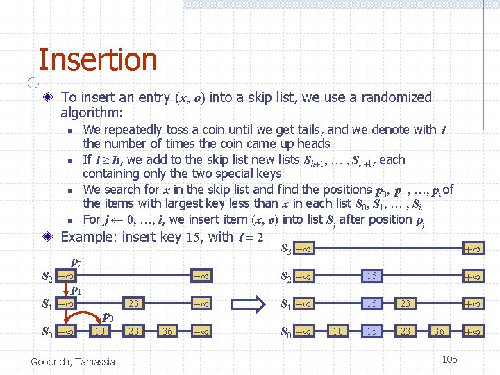
Insertion To insert an entry (x, o) into a skip list, we use a randomized algorithm: n n We repeatedly toss a coin until we get tails, and we denote with i the number of times the coin came up heads If i h, we add to the skip list new lists Sh+1, … , Si +1, each containing only the two special keys We search for x in the skip list and find the positions p 0, p 1 , …, pi of the items with largest key less than x in each list S 0, S 1, … , Si For j 0, …, i, we insert item (x, o) into list Sj after position pj Example: insert key 15, with i = 2 p 2 S 2 - p 1 S 1 - S 0 - p 0 10 Goodrich, Tamassia 23 23 36 S 3 - + + S 2 - 15 + S 1 - 15 23 + S 0 - 15 23 10 + + 36 105 +

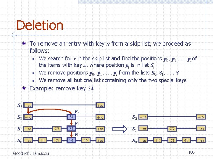
Deletion To remove an entry with key x from a skip list, we proceed as follows: n n n We the We We search for x in the skip list and find the positions p 0, p 1 , …, pi of items with key x, where position pj is in list Sj remove positions p 0, p 1 , …, pi from the lists S 0, S 1, … , Si remove all but one list containing only the two special keys Example: remove key 34 S 3 - p 2 S 2 - 34 S 1 - S 0 - + 12 Goodrich, Tamassia 23 34 p 1 p 0 45 + S 2 - + S 1 - + S 0 - + + 23 12 23 45 106 +

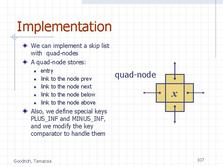
Implementation We can implement a skip list with quad-nodes A quad-node stores: n n n entry link to the the node prev next below above quad-node x Also, we define special keys PLUS_INF and MINUS_INF, and we modify the key comparator to handle them Goodrich, Tamassia 107

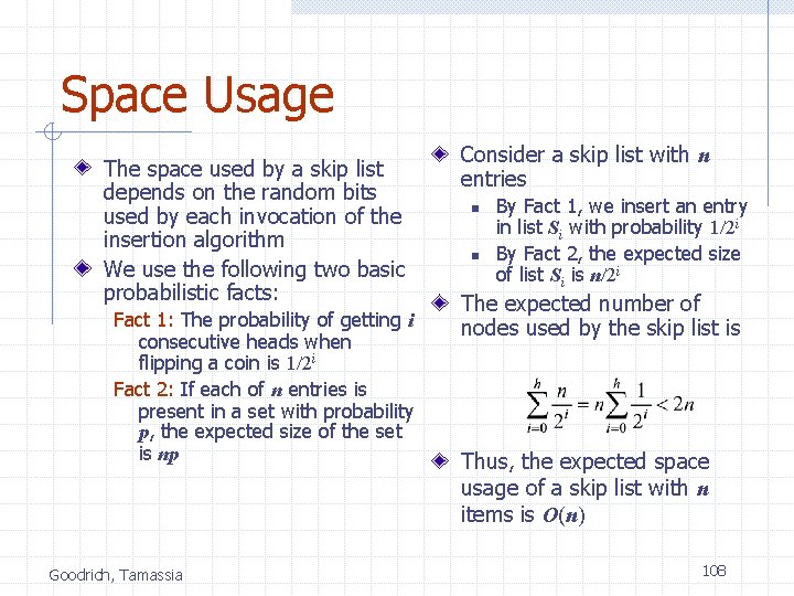
Space Usage The space used by a skip list depends on the random bits used by each invocation of the insertion algorithm We use the following two basic probabilistic facts: Fact 1: The probability of getting i consecutive heads when flipping a coin is 1/2 i Fact 2: If each of n entries is present in a set with probability p, the expected size of the set is np Goodrich, Tamassia Consider a skip list with n entries n n By Fact 1, we insert an entry in list Si with probability 1/2 i By Fact 2, the expected size of list Si is n/2 i The expected number of nodes used by the skip list is Thus, the expected space usage of a skip list with n items is O(n) 108

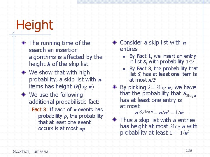
Height The running time of the search an insertion algorithms is affected by the height h of the skip list We show that with high probability, a skip list with n items has height O(log n) We use the following additional probabilistic fact: Fact 3: If each of n events has probability p, the probability that at least one event occurs is at most np Goodrich, Tamassia Consider a skip list with n entires n n By Fact 1, we insert an entry in list Si with probability 1/2 i By Fact 3, the probability that list Si has at least one item is at most n/2 i By picking i = 3 log n, we have that the probability that S 3 log n has at least one entry is at most n/23 log n = n/n 3 = 1/n 2 Thus a skip list with n entries has height at most 3 log n with probability at least 1 - 1/n 2 109

Search and Update Times The search time in a skip list is proportional to n n the number of drop-down steps, plus the number of scan-forward steps The drop-down steps are bounded by the height of the skip list and thus are O(log n) with high probability To analyze the scan-forward steps, we use yet another probabilistic fact: Fact 4: The expected number of coin tosses required in order to get tails is 2 Goodrich, Tamassia When we scan forward in a list, the destination key does not belong to a higher list n A scan-forward step is associated with a former coin toss that gave tails By Fact 4, in each list the expected number of scanforward steps is 2 Thus, the expected number of scan-forward steps is O(log n) We conclude that a search in a skip list takes O(log n) expected time The analysis of insertion and deletion gives similar results 110

Summary A skip list is a data structure for dictionaries that uses a randomized insertion algorithm In a skip list with n entries n n The expected space used is O(n) The expected search, insertion and deletion time is O(log n) Goodrich, Tamassia Using a more complex probabilistic analysis, one can show that these performance bounds also hold with high probability Skip lists are fast and simple to implement in practice 111