Time Series Analysis Definition A Time Series xt

Time Series Analysis

Definition A Time Series {xt : t T} is a collection of random variables usually parameterized by 1) the real line T = = (-∞, ∞) 2) the non-negative real line T = + = [0, ∞) 3) the integers T = = {…, -2, -1, 0, 1, 2, …} 4) the non-negative integers T = + = {0, 1, 2, …}

If xt is a vector, the collection of random vectors {xt : t T} is a multivariate time series or multi-channel time series. If t is a vector, the collection of random variables {xt : t T} is a multidimensional “time” series or spatial series. (with T = k= k-dimensional Euclidean space or a kdimensional lattice. )

Example of spatial time series

The project • Buoys are located in a grid across the Pacific ocean • Measuring – Surface temperature – Wind speed (two components) – Other measurements The data is being collected almost continuously The purpose is to study El Nino

Technical Note: The probability measure of a time series is defined by specifying the joint distribution (in a consistent manner) of all finite subsets of {xt : t T}. i. e. marginal distributions of subsets of random variables computed from the joint density of a complete set of variables should agree with the distribution assigned to the subset of variables.

The time series is Normal if all finite subsets of {xt : t T} have a multivariate normal distribution. Similar statements are true for multi-channel time series and multidimensional time series.

Definition: m(t) = mean value function of {xt : t T} = E[xt] for t T. s(t, s) = covariance function of {xt : t T} = E[(xt - m(t))(xs - m(s))] for t, s T.

For multichannel time series m(t) = mean vector function of {xt : t T} = E[xt] for t T and S(t, s) = covariance matrix function of {xt : t T} = E[(xt - m(t))(xs - m(s))′] for t, s T. The ith element of the k × 1 vector m(t) mi(t) =E[xit] is the mean value function of the time series {xit : t T} The i, jth element of the k × k matrix S(t, s) sij(t, s) =E[(xit - mi(t))(xjs - mj(s))] is called the cross-covariance function of the two time series {xit : t T} and {xjt : t T}

Definition: The time series {xt : t T} is stationary if the joint distribution of xt 1, xt 2, . . . , xtk is the same as the joint distribution of xt 1+h , xt 2+h , . . . , xtk+h for all finite subsets t 1, t 2, . . . , tk of T and all choices of h.

Definition: The multi-channel time series {xt : t T} is stationary if the joint distribution of xt 1, xt 2, . . . , xtk is the same as the joint distribution of xt 1+h , xt 2+h , . . . , xtk+h for all finite subsets t 1, t 2, . . . , tk of T and all choices of h.

Definition: The multidimensional time series {xt : t T} is stationary if the joint distribution of xt 1, xt 2, . . . , xtk is the same as the joint distribution of xt 1+h , xt 2+h , . . . , xtk+h for all finite subsets t 1, t 2, . . . , tk of T and all choices of h.

The distribution of observations at these points in time same as The distribution of observations at these points in time Time Stationarity

Some Implication of Stationarity If {xt : t T} is stationary then: 1. The distribution of xt is the same for all t T. 2. The joint distribution of xt, xt + h is the same as the joint distribution of xs, xs + h.

Implication of Stationarity for the mean value function and the covariance function If {xt : t T} is stationary then for t T. m(t) = E[xt] = m and for t, s T. s(t, s) = E[(xt - m)(xs - m)] = E[(xt+h - m)(xs+h - m)] = E[(xt-s - m)(x 0 - m)] with h = -s = s(t-s)

If the multi-channel time series{xt : t T} is stationary then for t T. m(t) = E[xt] = m and for t, s T S(t, s) = S(t-s) Thus for stationary time series the mean value function is constant and the covariance function is only a function of the distance in time (t – s)

If the multidimensional time series {xt : t T} is stationary then for t T. m(t) = E[xt] = m and for t, s T. s(t, s) = E[(xt - m)(xs - m)] = s(t-s) (called the Covariogram) Variogram V(t, s) = V(t - s) = Var[(xt - xs)] = E[(xt - xs)2] = Var[xt] + Var[xs] – 2 Cov[xt, xs] = 2[s(0) - s(t-s)]

Definition: r(t, s) = autocorrelation function of {xt : t T} = correlation between xt and xs. for t, s T. If {xt : t T} is stationary then r(h) = autocorrelation function of {xt : t T} = correlation between xt and xt+h.

Definition: The time series {xt : t T} is weakly stationary if: m(t) = E[xt] = m for all t T. and s(t, s) = s(t-s) for all t, s T. or r(t, s) = r(t-s) for all t, s T.

Examples Stationary time series

1. Let X denote a single random variable with mean m and standard deviation s. In addition X may also be Normal (this condition is not necessary) Let xt = X for all t T = { …, , -2, -1, 0, 1, 2, …} Then E[xt] = m = E[X] for t T and s(h) = E[(xt+h - m)(xt - m)] = Cov(xt+h, xt ) = E[(X - m)] = Var(X) = s 2 for all h.

Excel file illustrating this time series

2. Suppose {xt : t T} are identically distributed and uncorrelated (independent). T = { …, , -2, -1, 0, 1, 2, …} Then E[xt] = m = E[X] for t T and s(h) = E[(xt+h - m)(xt - m)] = Cov(xt+h, xt )

The auto correlation function: Comment: If m = 0 then the time series {xt : t T} is called a white noise time series. Thus a white noise time series consist of independent identically distributed random variables with mean 0 and common variance s 2

Excel file illustrating this time series

3. Suppose X 1, … , Xk and Y 1, Y 2, … , Yk are independent random variables with Let l 1, l 2, … lk denote k values in (0, p) For any t T = { …, , -2, -1, 0, 1, 2, …}

Excel file illustrating this time series

Then

Hence

Hence using cos(A – B) = cos(A) cos(B) + sin(A) sin(B) and

4. The Moving Average Time series of order q, MA(q) Let a 0 =1, a 2, … aq denote q + 1 numbers. Let {ut|t T} denote a white noise time series with variance s 2. – independent – mean 0, variance s 2. Let {xt|t T} be defined by the equation. Then {xt|t T} is called a Moving Average time series of order q. MA(q)

Excel file illustrating this time series

The mean The auto covariance function

The autocovariance function for an MA(q) time series The autocorrelation function for an MA(q) time series

5. The Autoregressive Time series of order p, AR(p) Let b 1, b 2, … bp denote p numbers. Let {ut|t T} denote a white noise time series with variance s 2. – independent – mean 0, variance s 2. Let {xt|t T} be defined by the equation. Then {xt|t T} is called a Autoregressive time series of order p. AR(p)

Excel file illustrating this time series

Comment: An Autoregressive time series is not necessarily stationary. Suppose {xt|t T} is an AR(1) time series satisfying the equation: where {ut|t T} is a white noise time series with variance s 2. i. e. b 1 = 1 and d = 0.

but and is not constant. A time series {xt|t T} satisfying the equation: is called a Random Walk.

Derivation of the mean, autocovariance function and autocorrelation function of a stationary Autoregressive time series We use extensively the rules of expectation

Assume that the autoregressive time series {xt|t T} be defined by the equation: is stationary. Let m = E(xt). Then

The Autocovariance function, s(h), of a stationary autoregressive time series {xt|t T}can be determined by using the equation: Thus

Hence where

Now

The equations for the autocovariance function of an AR(p) time series etc

Or using s(-h) = s(h) and for h > p

Use the first p + 1 equations to find s(0), s(1) and s(p) Then use To compute s(h) for h > p

The Autoregressive Time series of order p, AR(p) Let b 1, b 2, … bp denote p numbers. Let {ut|t T} denote a white noise time series with variance s 2. – independent – mean 0, variance s 2. Let {xt|t T} be defined by the equation. Then {xt|t T} is called a Autoregressive time series of order p. AR(p)

If the autoregressive time series {xt|t T} be defined by the equation: is stationary. Then

The Autocovariance function, s(h), of a stationary autoregressive time series {xt|t T} be defined by the equation: Satisfy the equations:

Yule Walker Equations and for h > p

Use the first p + 1 equations (the Yole-Walker Equations) to find s(0), s(1) and s(p) Then use To compute s(h) for h > p

The Autocorrelation function, r(h), of a stationary autoregressive time series {xt|t T}: The Yule walker Equations become:

and for h > p

To find r(h) and s(0): solve for r(1), …, r(p) Then for h > p

Example Consider the AR(2) time series: xt = 0. 7 xt – 1+ 0. 2 xt – 2 + 4. 1 + ut where {ut} is a white noise time series with standard deviation s = 2. 0 White noise ≡ independent, mean zero (normal) Find m, s(h), r(h)

To find r(h) solve the equations: or thus

for h > 2 This can be used in sequence to find: results

To find s(0) use: or = 17. 778

To find s(h) use: To find m use:

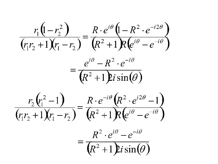
An explicit formula for r(h) Auto-regressive time series of order p.

Consider solving the difference equation: This difference equation can be solved by: Setting up the polynomial where r 1, r 2, … , rp are the roots of the polynomial b(x).

The difference equation has the general solution: where c 1, c 2, … , cp are determined by using the starting values of the sequence r(h).

Example: An AR(1) time series for h > 1 and

The difference equation Can also be solved by: Setting up the polynomial Then a general formula for r(h) is:

Example: An AR(2) time series for h > 1

Setting up the polynomial

Then a general formula for r(h) is: For h = 0 and h = 1. Solving for c 1 and c 2.

Solving for c 1 and c 2. and Then a general formula for r(h) is:

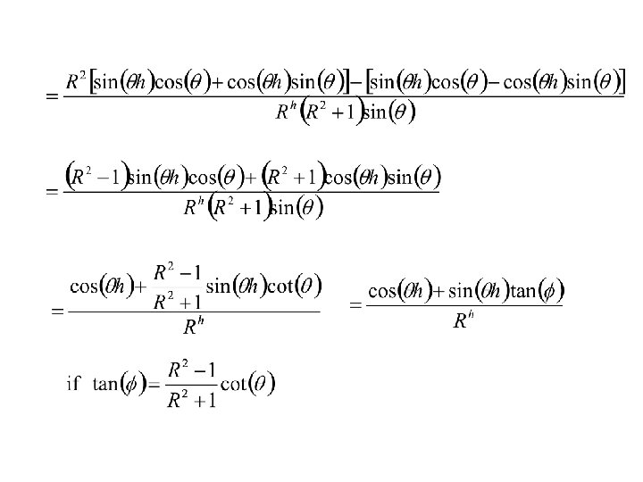
If are real and is a mixture of two exponentials

If are complex conjugates. Some important complex identities

The above identities can be shown using the power series expansions:

Some other trig identities:

Hence

a damped cosine wave

Example Consider the AR(2) time series: xt = 0. 7 xt – 1+ 0. 2 xt – 2 + 4. 1 + ut where {ut} is a white noise time series with standard deviation s = 2. 0 The correlation function found before using the difference equation: r(h) = 0. 7 r(h – 1) + 0. 2 r(h – 2)

Alternatively setting up the polynomial

Thus

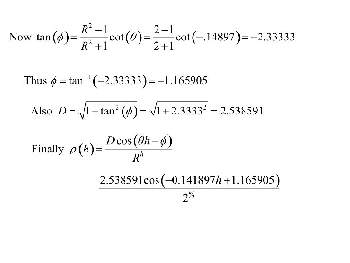
Another Example Consider the AR(2) time series: xt = 0. 2 xt – 1 - 0. 5 xt – 2 + 4. 1 + ut where {ut} is a white noise time series with standard deviation s = 2. 0 The correlation function found before using the difference equation: r(h) = 0. 2 r(h – 1) - 0. 5 r(h – 2)

Alternatively setting up the polynomial

Thus where and

a damped cosine wave

Conditions for stationarity Autoregressive Time series of order p, AR(p)

If b 1 = 1 and d = 0. The value of xt increases in magnitude and ut eventually becomes negligible. The time series {xt|t T} satisfies the equation: The time series {xt|t T} exhibits deterministic behaviour.

Let b 1, b 2, … bp denote p numbers. Let {ut|t T} denote a white noise time series with variance s 2. – independent – mean 0, variance s 2. Let {xt|t T} be defined by the equation. Then {xt|t T} is called a Autoregressive time series of order p. AR(p)

Consider the polynomial with roots r 1, r 2 , … , rp then {xt|t T} is stationary if |ri| > 1 for all i. If |ri| < 1 for at least one i then {xt|t T} exhibits deterministic behaviour. If |ri| ≥ 1 and |ri| = 1 for at least one i then {xt|t T} exhibits non-stationary random behaviour.

Special Cases: The AR(1) time Let {xt|t T} be defined by the equation.

Consider the polynomial with root r 1= 1/b 1 1. {xt|t T} is stationary if |r 1| > 1 or |b 1| < 1. 2. If |ri| < 1 or |b 1| > 1 then {xt|t T} exhibits deterministic behaviour. 3. If |ri| = 1 or |b 1| = 1 then {xt|t T} exhibits nonstationary random behaviour.

Special Cases: The AR(2) time Let {xt|t T} be defined by the equation.

Consider the polynomial where r 1 and r 2 are the roots of b(x) 1. {xt|t T} is stationary if |r 1| > 1 and |r 2| > 1. This is true if b 1+b 2 < 1 , b 2 –b 1 < 1 and b 2 > -1. These inequalities define a triangular region for b 1 and b 2. If |ri| < 1 or |b 1| > 1 then {xt|t T} exhibits deterministic behaviour. 3. If |ri| ≥ 1 for i = 1, 2 and |ri| = 1 for at least on i then {xt|t T} exhibits non-stationary random behaviour.

Patterns of the ACF and PACF of AR(2) Time Series In the shaded region the roots of the AR operator are complex b 2