Time Series 2 Thomas Schwarz SJ Time Series

Time Series 2 Thomas Schwarz SJ

Time Series • General Model of a time series: • • • Trend + seasonal(s) + remainder Trend seasonal(s) remainders Remainder can be modeled as a random walk

Trends • Example: Disposable Personal Income Massachusetts and Missouri • • from Federal Reserve Bank of St. Louis Need to check the raw data: Use separator df_ma = pd. read_csv('MAPCPI. csv', sep = ', ', ) df_ma. set_index('DATE', inplace = True)

Trends • Example continued: • We have two different files that we want to combine • Pandas has a merge function • Which needs to have a common column • Actually, merge implements an SQL-like join df = pd. merge(df_ma, df_mo, on='DATE')

Trends • We can now use linear recursion from statsmodels. formula. api import ols … model = ols("df. MOPCPI ~ df. MAPCPI", df). fit() inter, coef = model. params print(inter, coef) print(model. summary()) 900. 173966439816 0. 6894112036215065

Trends OLS Regression Results ======================================= Dep. Variable: df. MOPCPI R-squared: 0. 995 Model: OLS Adj. R-squared: 0. 995 Method: Least Squares F-statistic: 1. 710 e+04 Date: Fri, 03 Jul 2020 Prob (F-statistic): 1. 60 e-103 Time: 16: 40: 01 Log-Likelihood: -762. 99 No. Observations: 91 AIC: 1530. Df Residuals: 89 BIC: 1535. Df Model: 1 Covariance Type: nonrobust ======================================= coef std err t P>|t| [0. 025 0. 975] ---------------------------------------Intercept 900. 1740 147. 748 6. 093 0. 000 606. 601 1193. 747 df. MAPCPI 0. 6894 0. 005 130. 771 0. 000 0. 679 0. 700 ======================================= Omnibus: 0. 064 Durbin-Watson: 0. 066 Prob(Omnibus): 0. 969 Jarque-Bera (JB): 0. 069 Skew: 0. 051 Prob(JB): 0. 966 Kurtosis: 2. 911 Cond. No. 3. 69 e+04 =======================================

Trends • We then plot the result: plt. plot(df. MAPCPI, df. MOPCPI, '. ', alpha=0. 3) plt. plot(np. linspace(0, 75000), inter + coef*np. linsp plt. xlabel('MA') plt. ylabel('MO') plt. show()

Trends

Trends • We now look at the residual • We define it as an additional column df['residual'] = df. MOPCPI - inter-coef*df. MAPCPI

Trends • Showing the residual: • • Use xticks to make the x-axis readable And use fill to make the result clearer plt. plot(df. residual, 'k-') plt. xticks(['1930 -01 -01', '1950 -01 -01', '1970 -01 -01', ' plt. fill_between(df. index, 0, df. residual) plt. show()

Trends

Trends • This would be a bad regression for prediction!

Seasonal Dummy Variables • • Suppose you want to use linear regression Need to account for the effect of week-days • Introduce dummy variables t 1 t 2 t 3 t 4 t 5 t 6 t 7 3 Mon 1 0 0 0 Tue 0 1 0 0 0 Wed 0 0 1 0 0 Thu 0 0 0 1 0 0 0 Fri 0 0 1 0 0 Sat 0 0 0 1 0 Sun 0 0 0 1

Seasonal Dummy Variables • Use linear regression including the dummy variables

Seasonal Dummy Variables • Example: • Australian beer production (quarterly)

Seasonal Dummy Variables • Obviously, two different trends, 1955 - 1975 and 1975 -

Seasonal Dummy Variables • def Look at the original data: Time, Year, Quarter, Beer. Production 1, 1956, Q 1, 284 2, 1956, Q 2, 213 3, 1956, Q 3, 227 4, 1956, Q 4, 308 5, 1957, Q 1, 262 6, 1957, Q 2, 228 7, 1957, Q 3, 236 8, 1957, Q 4, 320 9, 1958, Q 1, 272 10, 1958, Q 2, 233 11, 1958, Q 3, 237 get_data(): 12, 1958, Q 4, 313 df_ab = pd. read_csv('Aus. Beer. csv', 13, 1959, Q 1, 261 14, 1959, Q 2, 227 sep = ', ', 15, 1959, Q 3, 250 parse_dates={'period': ['Year', 'Quarter']} 16, 1959, Q 4, 314 ) 17, 1960, Q 1, 286 • Need to parse time stamps from two different columns • Luckily, parse data is up to it df_ab = df_ab. set_index('period') return df_ab

Seasonal Dummy Variables • Aside: • When we draw the graph, need to select x-ticks def show(df_ab): plt. plot(df_ab['Beer. Production']) plt. plot(df_ab['pred']) plt. xticks(['1960 Q 1', '1980 Q 1', '2000 Q 1']) plt. show()

Seasonal Dummy Variables • First, linear regression just on beer production • without accounting for the influence of the quarters df_ab = get_data() df = df_ab. loc['1979 Q 1': ] y = df['Beer. Production'] x = df['Time'] model = ols("y~ x", df). fit() print(model. summary())

Seasonal Dummy Variables • This gives so-so values (as should be expected) OLS Regression Results ======================================= Dep. Variable: y R-squared: 0. 169 Model: OLS Adj. R-squared: 0. 163 Method: Least Squares F-statistic: 25. 26 Date: Fri, 03 Jul 2020 Prob (F-statistic): 1. 71 e-06 Time: 23: 43: 30 Log-Likelihood: -667. 55 No. Observations: 126 AIC: 1339. Df Residuals: 124 BIC: 1345. Df Model: 1 Covariance Type: nonrobust ======================================= coef std err t P>|t| [0. 025 0. 975] ---------------------------------------Intercept 545. 7075 19. 076 28. 606 0. 000 507. 950 583. 465 x -0. 6003 0. 119 -5. 026 0. 000 -0. 837 -0. 364 ======================================= Omnibus: 13. 659 Durbin-Watson: 2. 182 Prob(Omnibus): 0. 001 Jarque-Bera (JB): 15. 806 Skew: 0. 858 Prob(JB): 0. 000370 Kurtosis: 2. 740 Cond. No. 701. =======================================

Seasonal Dummy Variables • But already some nice trend • • Get the model parameters and add a new column with predicted values a, b = model. params df_ab['pred'] = a + b*df. Time Then display df_ab. dropna(inplace=True) plt. plot(df_ab['Beer. Production']) plt. plot(df_ab['pred']) plt. xticks(['1980 Q 1', '1985 Q 1', '1990 Q 1', '1995 Q 1', '2000 Q 1', '2005 Q 1', '2010 Q 1'], ['80', '85', '90', '95', '00', '05', '10'])

Seasonal Dummy Variables

Seasonal Dummy Variables • Now, let's try using seasonal dummy variables • Create four new columns def transform(df_ab): df_ab['s 1'] = [ 1 else 0 for df_ab['s 2'] = [ 1 else 0 for df_ab['s 3'] = [ 1 else 0 for df_ab['s 4'] = [ 1 else 0 for if 'Q 1' in df_ab. index[i] i in range(len(df_ab. index))] if 'Q 2' in df_ab. index[i] i in range(len(df_ab. index))] if 'Q 3' in df_ab. index[i] i in range(len(df_ab. index))] if 'Q 4' in df_ab. index[i] i in range(len(df_ab. index))]

Seasonal Dummy Variables • Create a slice since 1979 df_ab = get_data() transform(df_ab) df = df_ab. loc['1979 Q 1': ]

Seasonal Dummy Variables • Set up the model including the seasonal parameters y = df['Beer. Production'] x = df['Time'] x 1 = df['s 1'] x 2 = df['s 2'] x 3 = df['s 3'] x 4 = df['s 4'] model = ols("y~ x", df). fit() print(model. summary()) a, b, b 1, b 2, b 3, b 4 = model. params print(a, b, b 1, b 2, b 3, b 4)

Seasonal Dummy Variables OLS Regression Results ======================================= Dep. Variable: y R-squared: 0. 887 Model: OLS Adj. R-squared: 0. 883 Method: Least Squares F-statistic: 237. 6 Date: Fri, 03 Jul 2020 Prob (F-statistic): 2. 70 e-56 Time: 23: 56: 27 Log-Likelihood: -541. 83 No. Observations: 126 AIC: 1094. Df Residuals: 121 BIC: 1108. Df Model: 4 Covariance Type: nonrobust ======================================= coef std err t P>|t| [0. 025 0. 975] ---------------------------------------Intercept 437. 5337 5. 696 76. 809 0. 000 426. 256 448. 811 x -0. 6058 0. 045 -13. 586 0. 000 -0. 694 -0. 517 x 1 107. 4220 3. 124 34. 390 0. 000 101. 238 113. 606 x 2 65. 4965 3. 143 20. 837 0. 000 59. 273 71. 720 x 3 81. 4240 3. 156 25. 804 0. 000 75. 177 87. 671 x 4 183. 1911 3. 175 57. 697 0. 000 176. 905 189. 477 ======================================= Omnibus: 20. 235 Durbin-Watson: 1. 948 Prob(Omnibus): 0. 000 Jarque-Bera (JB): 34. 949 Skew: 0. 731 Prob(JB): 2. 58 e-08 Kurtosis: 5. 126 Cond. No. 4. 40 e+17 =======================================

Seasonal Dummy Variables • Add a new column for the prediction • • df_ab['pred'] = a + b*df. Time +b 1*df. s 1+b 2*df. s 2 df_ab. dropna(inplace=True) And plot raw data and prediction values plt. plot(df_ab['Beer. Production']) plt. plot(df_ab['pred'], alpha = 0. 5) plt. xticks(['1980 Q 1', '1985 Q 1', '1990 Q 1', '1995 Q 1', '2000 Q 1', '2005 Q 1', '2010 Q 1'], ['80', '85', '90', '95', '00', '05', '10']) plt. show()

Seasonal Dummy Variables

Seasonal Dummy Variables • Why are we not doing better? • We only have time and season as explanatory variables • Temperature and economy could also explain beer consumption • And maybe exports?

Seasonal Dummy Variables • Let's look at the average error of the prediction • Add one more column to the data frame • • df_ab['res'] = (df_ab['Beer. Production']df_ab['pred'])/df_ab['Beer. Production'] And display

Seasonal Dummy Variables • Shows that we are historically with 10% of the linear regression calculated value

Seasonal Dummy Variables • We can also look at how well the prediction works plt. scatter(df_ab['Beer. Production'][df_ab['s 1']==1], df_ab['pred'][df_ab['s 1']==1], alpha = 0. 5, c = 'red', label='Q 1') plt. scatter(df_ab['Beer. Production'][df_ab['s 2']==1], df_ab['pred'][df_ab['s 2']==1], alpha = 0. 5, c = 'green', label='Q 2') plt. scatter(df_ab['Beer. Production'][df_ab['s 3']==1], df_ab['pred'][df_ab['s 3']==1], alpha = 0. 5, c = 'blue', label='Q 3') plt. scatter(df_ab['Beer. Production'][df_ab['s 4']==1], df_ab['pred'][df_ab['s 4']==1], alpha = 0. 5, c = 'cyan', label='Q 4') plt. legend() plt. show()

Seasonal Dummy Variables

Classical Decomposition • Simple method with periods of m on • • quarters: m=4, business weeks: m=5, years: m = 365 Additive decomposition: • • • Use moving average of size 2 m (or m) to estimate • Residual is what is left Calculate the "detrended" series Seasonal component is the average over all values for that period

Classical Decomposition • Problems with classical decomposition: • Trend cycle not available for the first or last times without extrapolation • • Rapid rises and falls are smoothed out too much Assumes seasonal components repeat • • Counter-example: • Used to be that electricity consumption peaked in the winter (heating) • Now peaks in the summer (air-conditioning) Really difficult to deal with extra-ordinary events (strikes, weather, catastrophes, …)

Classical Decomposition • Implemented in statsmodels from statsmodels. tsa. seasonal import seasonal_decompose • • • Needs a time series x Needs a model: "additive" (default), "multiplicative Can give filtering weights Period (if x not Pandas with frequency) two-sided: method used for filtering extrapolate_trend: non-zero value or 'freq' to extrapolate • Otherwise, Na. N values

Classical Decomposition • Example: Australian beer production (again) def get_data(): df_ab = pd. read_csv('Aus. Beer. csv', sep = ', ', parse_dates={'period': ['Year', 'Quarter']} ) df_ab = df_ab. set_index('period') return df_ab

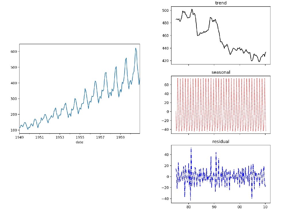
Classical Decomposition • Limit to values after 1975 • • df = get_data()['1975 Q 1': ] Call decomposition • • result = seasonal_decompose( df['Beer. Production'], model = 'additive', period = 4, extrapolate_trend = 3) result has components trend, seasonal, resid

Classical Decomposition • Show results: def show(result): fig, axs = plt. subplots(3, sharex=True, figsize=(5, 10)) axs[0]. plot(result. trend, 'k-') axs[1]. plot(result. seasonal, 'r: ') axs[2]. plot(result. resid, 'b-. ') axs[0]. set_title('trend') axs[1]. set_title('seasonal') axs[2]. set_title('residual') axs[2]. set_xticks(['1980 Q 1', '1990 Q 1', '2000 Q 1', '2010 Q 1']) axs[2]. set_xticklabels(['80', '90', '00', '10']) plt. show()

• • • Can extrapolate the trend Add seasonal Use residual as a measure of uncertainty

Classical Decomposition • airline passengers result = seasonal_decompose(df. Passengers, model = 'additive', period = 14, extrapolate_trend = 'freq' )

Better Decompositions • Decomposition has had a 100 year history • • Better decompositions allow seasonal values to vary Seasonal Decomposition using LOESS (STL) • LOESS is based on estimating the trend with a range of functions within a certain window

Better Decompositions • STL is implemented in statsmodels • • from statsmodels. tsa. seasonal import STL Uses the assumed cyclicity as input (periods)

Better Decompositions • Example: Australian Beer: df = get_data()['1975 Q 1': ] stl = STL(df['Beer. Production'], period=4, robust=False) result = stl. fit() • Result is a triple of trend, seasonal, and resid

Better Decompositions robust not robust

Better Decompositions airline passengers not robust

Better Decompositions • Holt's linear trend method: • Simple exponential smoothing for data with trend • • Estimates series at time t using estimates of the slope obtained as a weighted average Holt-Winter's Seasonal Method • Adds a seasonal component

Better Decompositions • Implemented in statsmodels • • from statsmodels. tsa. holtwinters import Exponent Produces a fitted value (fit) and allows predictions df = get_data() esm = esm(df['Passengers'], seasonal='mul', seasonal_periods=12 ) result = esm. fit()

Better Decompositions • Airline Example (multiplicative fit)

Better Decompositions • Airline Example additive seasonality

Stationary Time Series • Properties do not depend on the time at which the series is observed • • No trend, no seasonality But could be cyclic if cycles have no fixed length

Stationary Time Series • Example: • Google High stock value is not stationary

Stationary Time Series • But it's daily change is

Stationary Time Series • Use shift in order to obtain the differences def get_google_data(): my_df = pd. read_csv('. . /Pandas/google. csv', parse_dates=[0], index_col=0, converters={ 'Close': my_converter, 'Volume': convert_volume} ) print(my_df. info()) #my_df. High. plot() (my_df. shift(1). High - my_df. High). plot() plt. show() return my_df

Stationary Time Series • This is typical • Differencing • • Make a non-stationary time series stationary Might have to be repeated several times

Stationary Time Series • Can look at the Auto-Correlation Function • • How does the value of a time series relate to the values shifted by m periods Implemented in Pandas as autocorr(lag = m)

Stationary Time Series • Example: google change my_df = get_google_data() for i in range(20): print(i, (my_df. shift(1). High - my_df. High). autocorr(lag=i)) 0 1 2 3 4 5 6 7 8 0. 99999999 0. 12080309541084427 -0. 035334997385017435 -0. 048524948019570004 -0. 05560693878878337 -0. 0064797046657102605 0. 011124537759089287 -0. 03901650231472603 -0. 012520771888603816

Stationary Time Series • One version in statsmodels from statsmodels. tsa. stattools import acf, pacf • Calculates ACF as a numpy array my_df = get_google_data() google = (my_df. shift(1) - my_df). dropna(axis=0) my_acf = acf(google. High, fft = False) fig, ax = plt. subplots(1) ax. plot(my_acf)

Stationary Time Series

Stationary Time Series • A graphical version is also available: • import statsmodels. graphics. tsaplots as sgt. plot_acf(google. High, unbiased = True, zero=False, lags = 40)

Stationary Time Series

Stationary Time Series • If we apply the same methodology to the original data • Much more autocorrelation

Stationary Time Series • For lag = 2, the value is mostly because of the correlation between lag = 1 • Use pacm instead • Calculates only the auto-correlation not explained by auto-correlation for smaller lags sgt. plot_pacf(my_df. High, lags = 40)

Stationary Time Series

Stationary Time Series • Autoregression Models • Forecast variable of interest using linear combination of past values of the variable • • With "white error" Autoregressive Model of order

Stationary Time Series • Moving average models • Uses past forecast errors • with white noise

Stationary Time Series • ARIMA models • Auto. Regressive Integrated Moving Average • Differenced value at t is • autoregressive part of order p • d times differenciated • moving average of order q • ARIMA(p, d, q)

Stationary Time Series • Can use statsmodels • from statsmodels. tsa. arima_model import ARIMA • Specify degree of ARIMA model and print out its parameters • Display residual model = ARIMA(my_df. High, order=(1, 1, 0)) model_fit = model. fit(disp=0) print(model_fit. summary()) residuals = pd. Data. Frame(model_fit. resid) residuals. plot(label='residual') plt. show()

Stationary Time Series

Seasonal Time Series • It is possible to extend ARIMA to include a seasonal component • In which case we could even put in a trend from statsmodels. tsa. statespace. sarimax import SARIMAX df = get_data() my_order = (1, 1, 1) my_seasonal_order=(1, 1, 1, 12) model = SARIMAX(endog = df. Passengers, order = my_order, seasonal_order = my_seasonal_order) results = model. fit() print(results. summary()) results. resid. plot() plt. show()

Stationary Time Series

Stationary Time Series