Time series Decomposition Additive Model Farideh DehkordiVakil Classical

Time series Decomposition Additive Model Farideh Dehkordi-Vakil

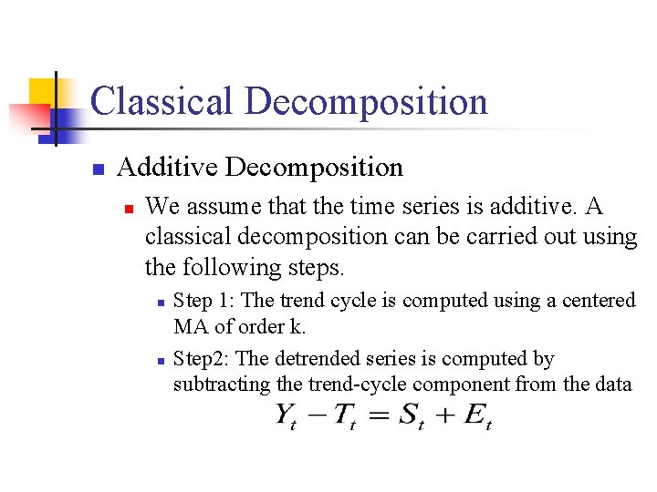
Classical Decomposition n Additive Decomposition n We assume that the time series is additive. A classical decomposition can be carried out using the following steps. n n Step 1: The trend cycle is computed using a centered MA of order k. Step 2: The detrended series is computed by subtracting the trend-cycle component from the data

Classical Decomposition n Additive Decomposition n n Step 3: In classical decomposition we assume the seasonal component is constant from year to year. So we the average of the detrended value for a given month (for monthly data) and given quarter (for quarterly data) will be the seasonal index for the corresponding month or quarter. Step 4: the irregular series Et is computed by simply subtracting the estimated seasonality, and trendcycle from the original data.

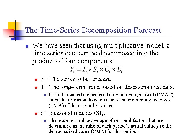
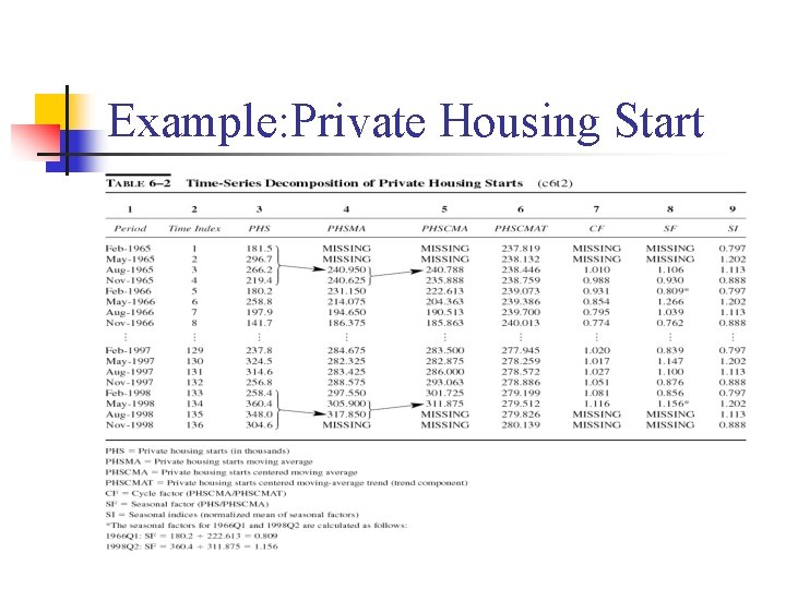
The Time-Series Decomposition Forecast n We have seen that using multiplicative model, a time series data can be decomposed into the product of four components: n n Y= The series to be forecast. T= The long–term trend based on deseasonalized data. n n It is often called the centered moving-average trend (CMAT) since the deseasonalized data are centered moving averages (CMA) of the original Y values. S = Seasonal indexes (SI). n These are normalize average of seasonal factors that are determined as the ratio of each period’s actual value y to the deseaonalized value (CMA) for that period.

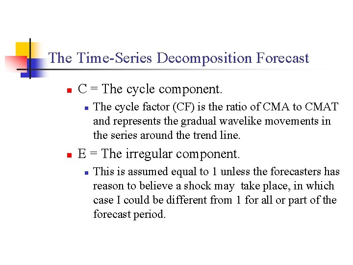
The Time-Series Decomposition Forecast n C = The cycle component. n n The cycle factor (CF) is the ratio of CMA to CMAT and represents the gradual wavelike movements in the series around the trend line. E = The irregular component. n This is assumed equal to 1 unless the forecasters has reason to believe a shock may take place, in which case I could be different from 1 for all or part of the forecast period.

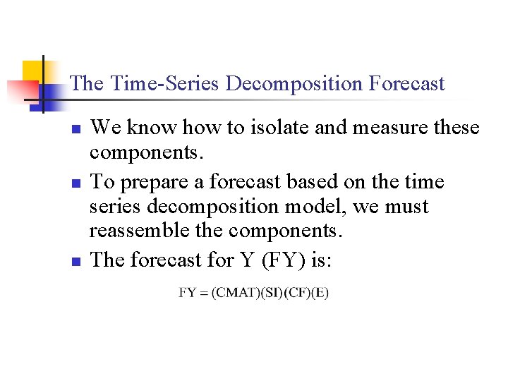
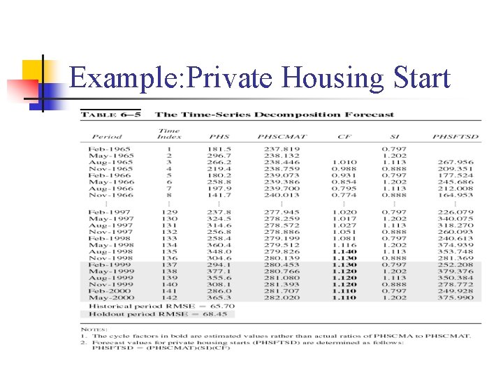
The Time-Series Decomposition Forecast n n n We know how to isolate and measure these components. To prepare a forecast based on the time series decomposition model, we must reassemble the components. The forecast for Y (FY) is:

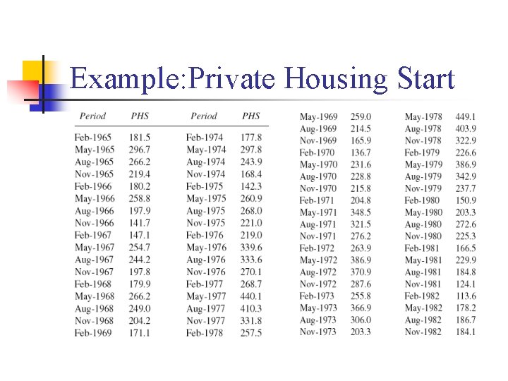
Example: Private Housing Start

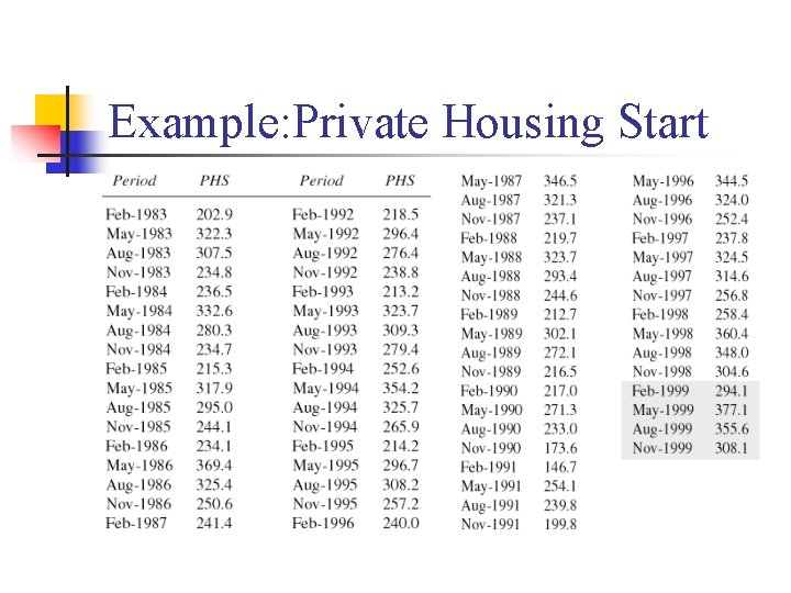
Example: Private Housing Start

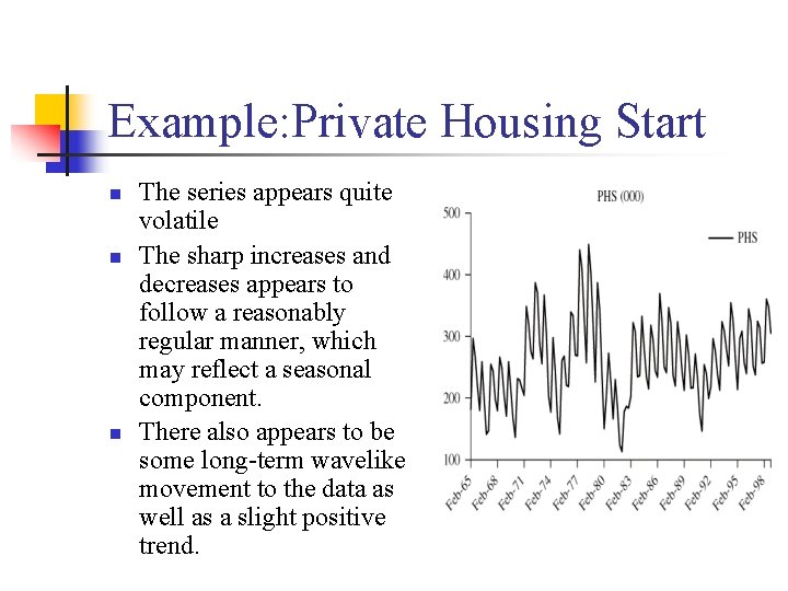
Example: Private Housing Start n n n The series appears quite volatile The sharp increases and decreases appears to follow a reasonably regular manner, which may reflect a seasonal component. There also appears to be some long-term wavelike movement to the data as well as a slight positive trend.

Example: Private Housing Start

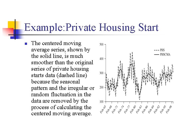
Example: Private Housing Start n The centered moving average series, shown by the solid line, is much smoother than the original series of private housing starts data (dashed line) because the seasonal pattern and the irregular or random fluctuation in the data are removed by the process of calculating the centered moving average.

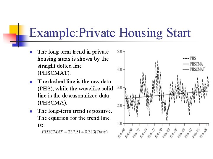
Example: Private Housing Start n n n The long term trend in private housing starts is shown by the straight dotted line (PHSCMAT). The dashed line is the raw data (PHS), while the wavelike solid line is the deseasonalized data (PHSCMA). The long-term trend is positive. The equation for the trend line is:

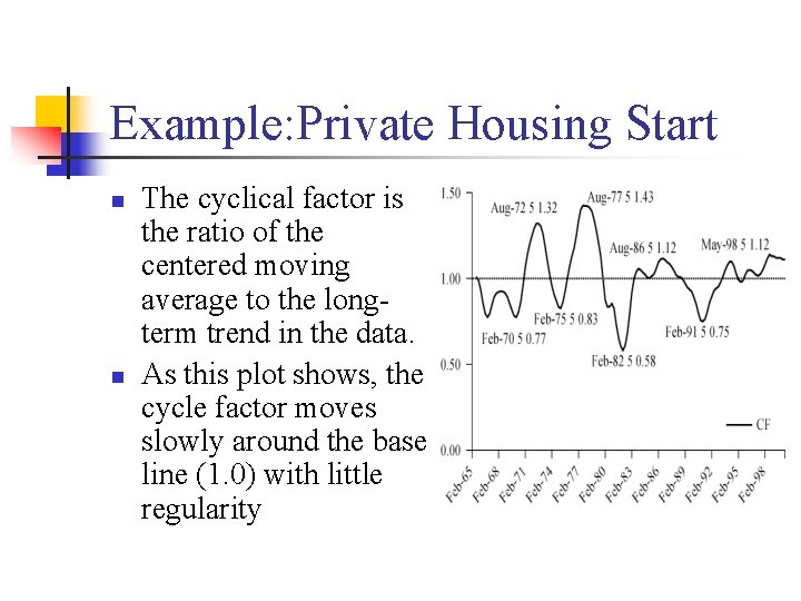
Example: Private Housing Start n n The cyclical factor is the ratio of the centered moving average to the longterm trend in the data. As this plot shows, the cycle factor moves slowly around the base line (1. 0) with little regularity

Example: Private Housing Start

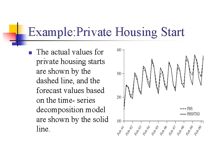
Example: Private Housing Start n The actual values for private housing starts are shown by the dashed line, and the forecast values based on the time- series decomposition model are shown by the solid line.

The Time-Series Decomposition Forecast n n Because the time series decomposition models do not involve a lot of mathematics or statistics, they are relatively easy to explain to the end user. This is a major advantage because if the end user has an appreciation of how the forecast was developed, he or she may have more confidence in its use for decision making.