Fast Shapelets All Figures in Higher Resolution 0

Fast Shapelets: All Figures in Higher Resolution

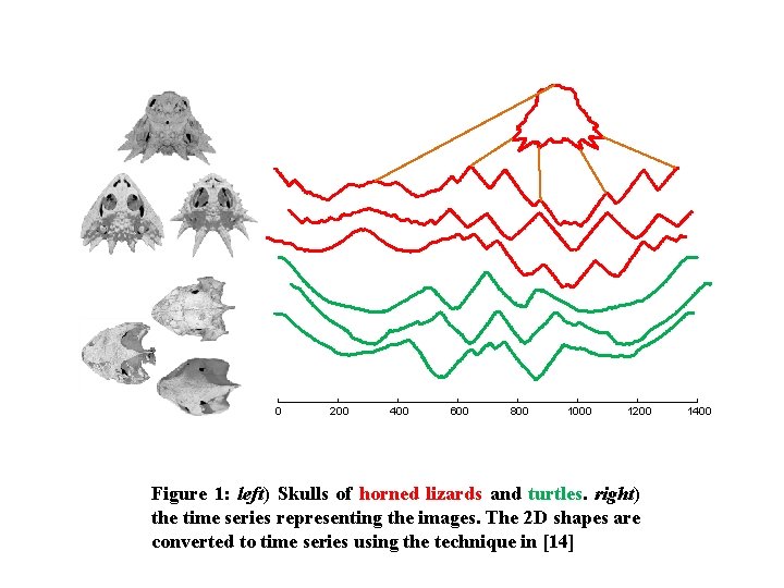
0 200 400 600 800 1000 1200 Figure 1: left) Skulls of horned lizards and turtles. right) the time series representing the images. The 2 D shapes are converted to time series using the technique in [14] 1400

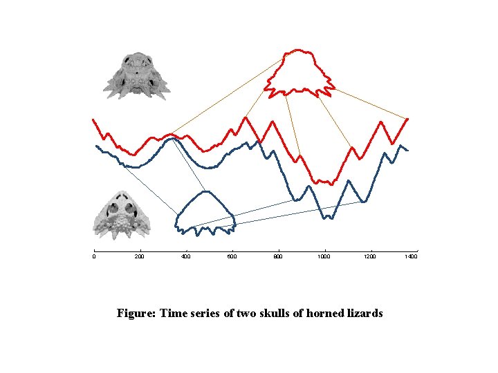
0 200 400 600 800 1000 1200 Figure: Time series of two skulls of horned lizards 1400

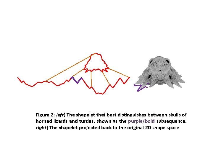
Figure 2: left) The shapelet that best distinguishes between skulls of horned lizards and turtles, shown as the purple/bold subsequence. right) The shapelet projected back to the original 2 D shape space

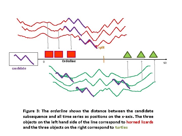
split 0 Orderline candidate Figure 3: The orderline shows the distance between the candidate subsequence and all time series as positions on the x-axis. The three objects on the left hand side of the line correspond to horned lizards and the three objects on the right correspond to turtles ∞

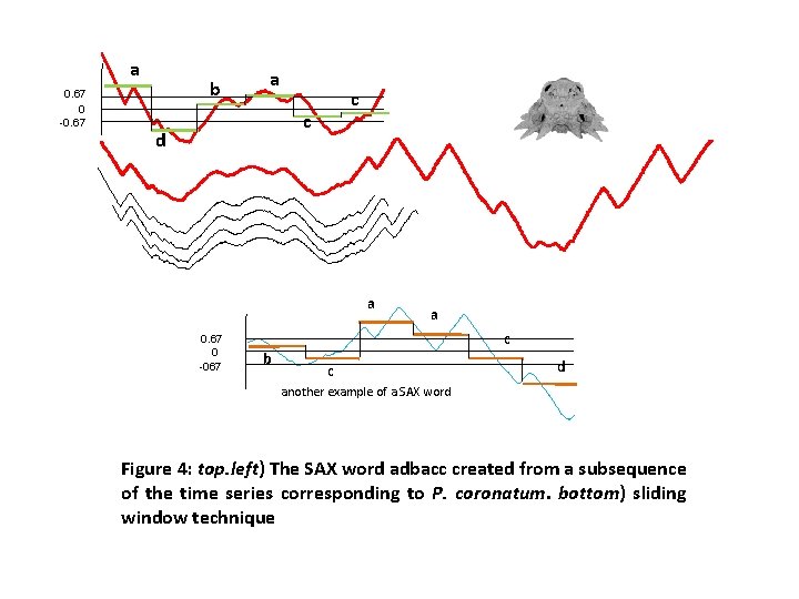
a 0. 67 0 -0. 67 b a c c d a 0. 67 0 -067 a c b c d another example of a SAX word Figure 4: top. left) The SAX word adbacc created from a subsequence of the time series corresponding to P. coronatum. bottom) sliding window technique

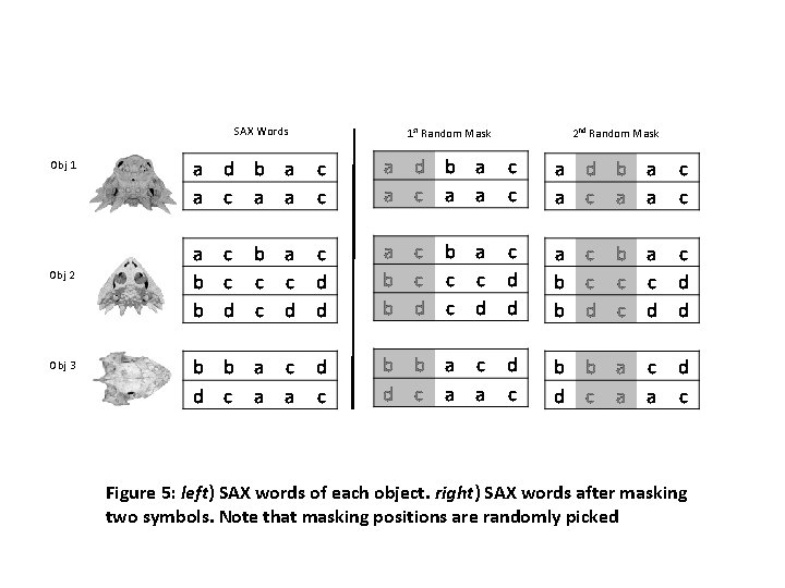
SAX Words 1 st Random Mask 2 nd Random Mask Obj 1 Obj 2 Obj 3 Figure 5: left) SAX words of each object. right) SAX words after masking two symbols. Note that masking positions are randomly picked

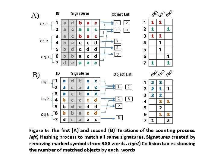
ID A) Signatures Obj 1 Object List 1 2 1 3 j 1 bj 2 bj 3 b O O O 2 Obj 2 2 3 Obj 3 B) ID Signatures Object List j 1 bj 2 bj 3 b O Obj 1 Obj 2 1 2 2 3 2 Obj 3 3 Figure 6: The first (A) and second (B) iterations of the counting process. left) Hashing process to match all same signatures. Signatures created by removing marked symbols from SAX words. right) Collision tables showing the number of matched objects by each words

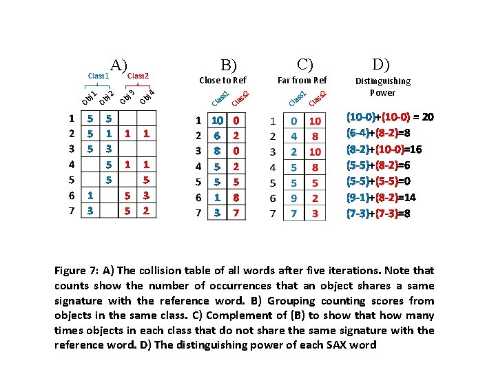
Class 1 j Ob 1 A)Class 2 j Ob 3 j Ob C) B) Close to Ref 4 s 1 as Cl s 2 C las D) Far from Ref s 1 as Cl s 2 as Cl Distinguishing Power Figure 7: A) The collision table of all words after five iterations. Note that counts show the number of occurrences that an object shares a same signature with the reference word. B) Grouping counting scores from objects in the same class. C) Complement of (B) to show that how many times objects in each class that do not share the same signature with the reference word. D) The distinguishing power of each SAX word

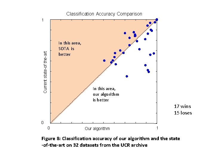
Classification Accuracy Comparison 1 Current state-of the-art In this area, SOTA is better In this area, our algorithm is better 17 wins 15 loses 0 0 Our algorithm 1 Figure 8: Classification accuracy of our algorithm and the state -of-the-art on 32 datasets from the UCR archive

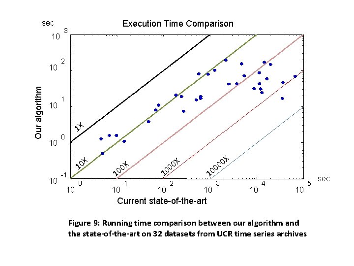
sec 10 Our algorithm 10 10 Execution Time Comparison 3 2 1 1 X 0 X 10 -1 10 0 X 00 1 10 10 X 00 2 10 10 0 00 3 X 10 4 10 Current state-of-the-art Figure 9: Running time comparison between our algorithm and the state-of-the-art on 32 datasets from UCR time series archives 5 sec

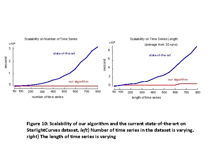
Scalability on Number of Time Series Scalability on Time Series Length x 103 x 104 3 8 seccond state-of-the-art seccond (average from 30 runs) 2 1 state-of-the-art 6 4 2 our algorithm 0 0 50 100 200 300 400 500 number of time series 600 700 800 50 100 200 300 400 500 600 700 length of time series Figure 10: Scalability of our algorithm and the current state-of-the-art on Starlight. Curves dataset. left) Number of time series in the dataset is varying. right) The length of time series is varying 800

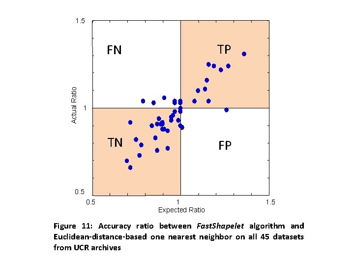
Actual Ratio 1. 5 FN TP TN FP 1 0. 5 1 Expected Ratio 1. 5 Figure 11: Accuracy ratio between Fast. Shapelet algorithm and Euclidean-distance-based one nearest neighbor on all 45 datasets from UCR archives

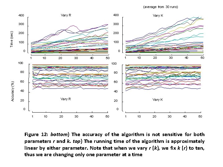
(average from 30 runs) Time (sec) 400 Vary R 400 300 200 100 0 0 1 Accuracy (%) Vary K 10 20 30 40 1 50 100 80 80 60 60 40 40 Vary R 20 10 30 40 50 Vary K 20 0 1 10 20 30 40 50 Figure 12: bottom) The accuracy of the algorithm is not sensitive for both parameters r and k. top) The running time of the algorithm is approximately linear by either parameter. Note that when we vary r (k), we fix k (r) to ten, thus we are changing only one parameter at a time

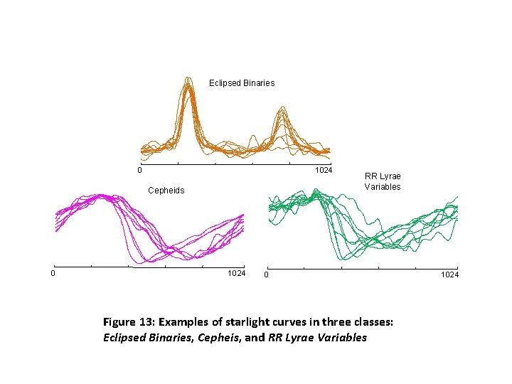
Eclipsed Binaries 0 1024 Cepheids 0 1024 RR Lyrae Variables 0 Figure 13: Examples of starlight curves in three classes: Eclipsed Binaries, Cepheis, and RR Lyrae Variables 1024

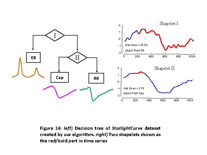
Shapelet I 2 1 I 0 dist thres = 15. 58 -1 II EB object from RR -2 0 200 400 RR 800 1024 Shapelet II 2 Cep 600 1 0 dist thres = 5. 79 -1 object from Cep -2 0 200 400 600 Figure 14: left) Decision tree of Starlight. Curve dataset created by our algorithm. right) Two shapelets shown as the red/bold part in time series 800 1024

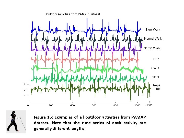
Outdoor Activities from PAMAP Dataset Slow Walk Normal Walk Nordic Walk Run Cycle Soccer 3 Rope Jump 0 -3 0 200 400 600 800 1000 Figure 15: Examples of all outdoor activities from PAMAP dataset. Note that the time series of each activity are generally different lengths 1100

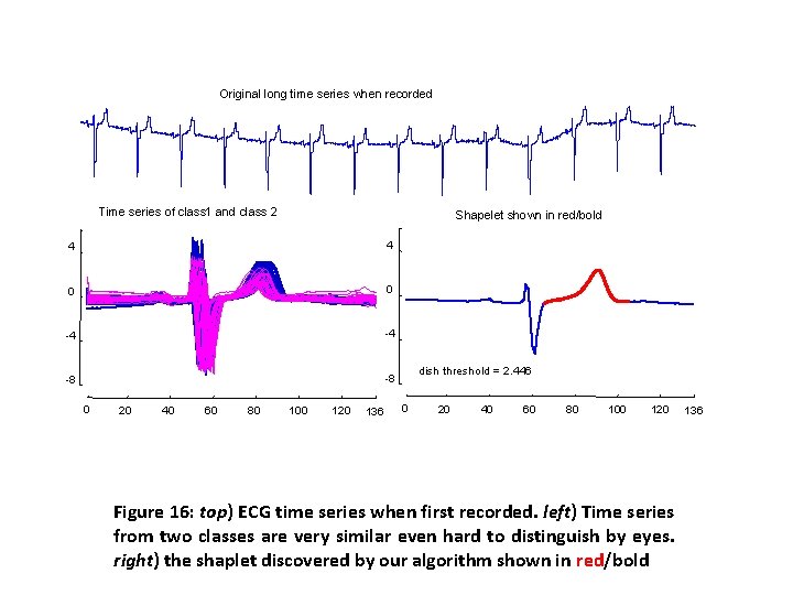
Original long time series when recorded Time series of class 1 and class 2 Shapelet shown in red/bold 4 4 0 0 -4 -4 -8 -8 0 20 40 60 80 100 120 136 dish threshold = 2. 446 0 20 40 60 80 100 120 Figure 16: top) ECG time series when first recorded. left) Time series from two classes are very similar even hard to distinguish by eyes. right) the shaplet discovered by our algorithm shown in red/bold 136