Introduction to Time Series Is it Time Series

Introduction to Time Series Is it Time Series Data? ¡ Is it Cross Sectional Data? ¡ Is it Panel (Pooled Data)? ¡

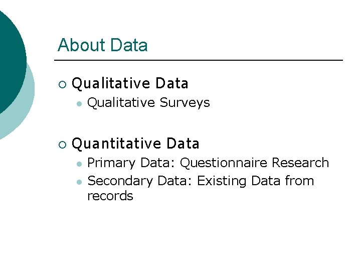
About Data ¡ Qualitative Data l ¡ Qualitative Surveys Quantitative Data l l Primary Data: Questionnaire Research Secondary Data: Existing Data from records

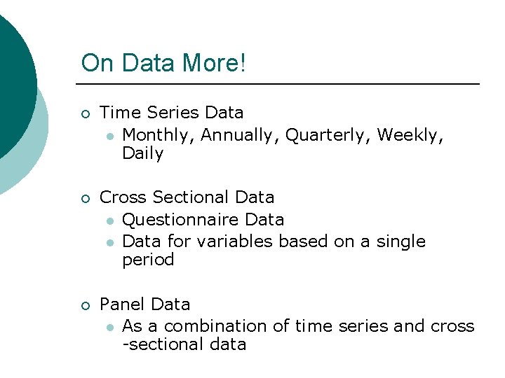
On Data More! ¡ Time Series Data l Monthly, Annually, Quarterly, Weekly, Daily ¡ Cross Sectional Data l Questionnaire Data l Data for variables based on a single period ¡ Panel Data l As a combination of time series and cross -sectional data

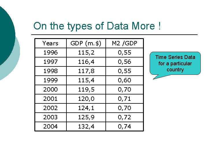
On the types of Data More ! Years GDP (m. $) M 2 /GDP 1996 115, 2 0, 55 1997 116, 4 0, 56 1998 117, 8 0, 55 1999 115, 4 0, 60 2000 119, 5 0, 70 2001 120, 0 0, 71 2002 124, 1 0, 70 2003 125, 9 0, 72 2004 132, 4 0, 74 Time Series Data for a particular country

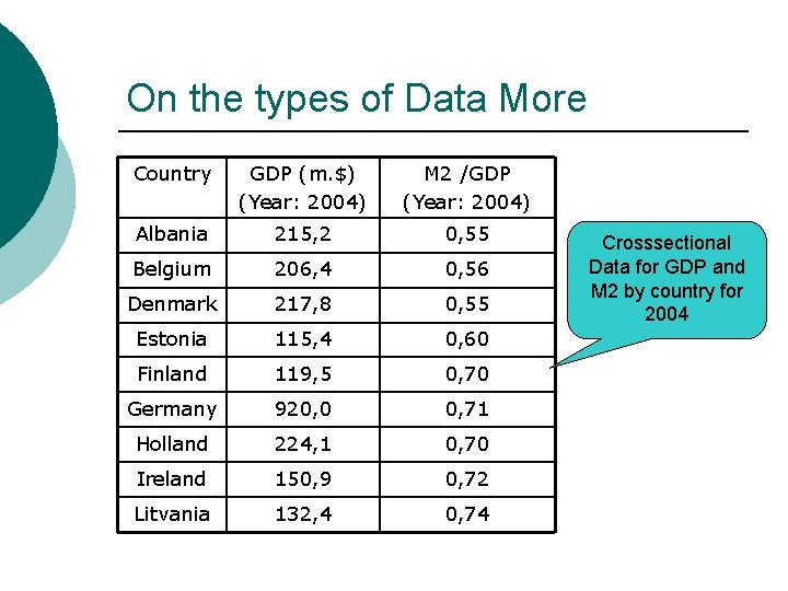
On the types of Data More Country GDP (m. $) (Year: 2004) M 2 /GDP (Year: 2004) Albania 215, 2 0, 55 Belgium 206, 4 0, 56 Denmark 217, 8 0, 55 Estonia 115, 4 0, 60 Finland 119, 5 0, 70 Germany 920, 0 0, 71 Holland 224, 1 0, 70 Ireland 150, 9 0, 72 Litvania 132, 4 0, 74 Crosssectional Data for GDP and M 2 by country for 2004

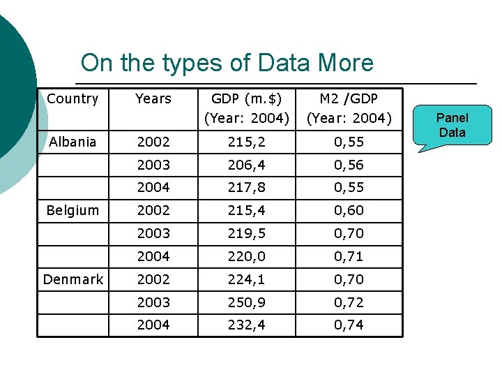
On the types of Data More Country Albania Belgium Denmark Years GDP (m. $) (Year: 2004) M 2 /GDP (Year: 2004) 2002 215, 2 0, 55 2003 206, 4 0, 56 2004 217, 8 0, 55 2002 215, 4 0, 60 2003 219, 5 0, 70 2004 220, 0 0, 71 2002 224, 1 0, 70 2003 250, 9 0, 72 2004 232, 4 0, 74 Panel Data

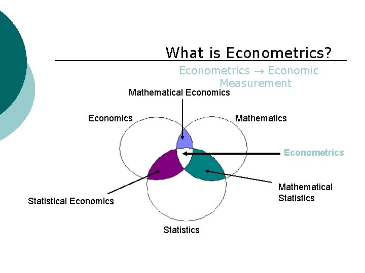
What is Econometrics? Econometrics Economic Measurement Mathematical Economics Mathematics Econometrics Mathematical Statistics Statistical Economics Statistics

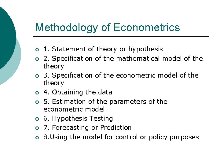
Methodology of Econometrics ¡ ¡ ¡ ¡ 1. Statement of theory or hypothesis 2. Specification of the mathematical model of theory 3. Specification of the econometric model of theory 4. Obtaining the data 5. Estimation of the parameters of the econometric model 6. Hypothesis Testing 7. Forecasting or Prediction 8. Using the model for control or policy purposes

Stationarity Empirical work based on time series data assumes that the underlying time series is stationary. ¡ Otherwise, are econometric results spurious or non-sense? ¡ Then, what is Stationarity? ¡

Definition of “Stationarity” A time series might be equal to its value plus a purely random shock (or error term). Thus, this means a random walk phenomenon (Especially in financial time series). ¡ Thus, the relationship between two series need to be the one with “stationarity” charactetistic. ¡

A Stationary Stochastic Process A random or stochastic process is a collection of random variables ordered in time. ¡ Thus, a type stochastic process is the so-called stationary stochastic process. ¡

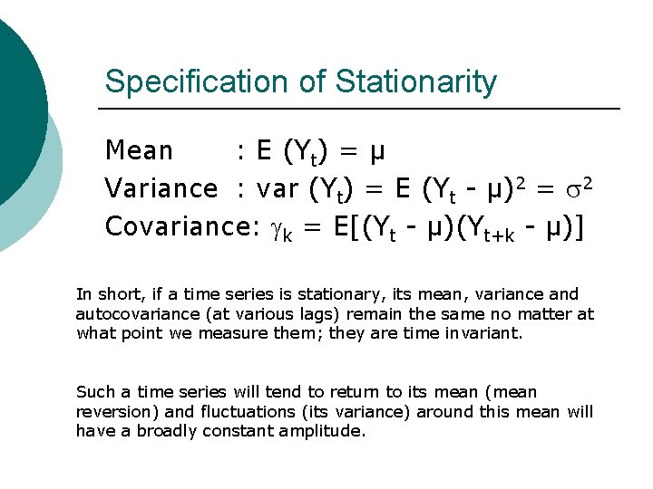
Specification of Stationarity Mean : E (Yt) = µ Variance : var (Yt) = E (Yt - µ)2 = 2 Covariance: k = E[(Yt - µ)(Yt+k - µ)] In short, if a time series is stationary, its mean, variance and autocovariance (at various lags) remain the same no matter at what point we measure them; they are time invariant. Such a time series will tend to return to its mean (mean reversion) and fluctuations (its variance) around this mean will have a broadly constant amplitude.

Tests of Stationarity ¡ 1. Graphical Analysis ¡ 2. Autocorrelation Function (ACF) and Correlogram ¡ 3. The Unit Root Tests (The main Focus of “all the tests of Stationarity”)

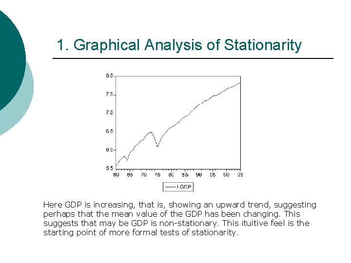
1. Graphical Analysis of Stationarity Here GDP is increasing, that is, showing an upward trend, suggesting perhaps that the mean value of the GDP has been changing. This suggests that may be GDP is non-stationary. This ituitive feel is the starting point of more formal tests of stationarity.

2. Autocorrelation Function (ACF) and Correlogram

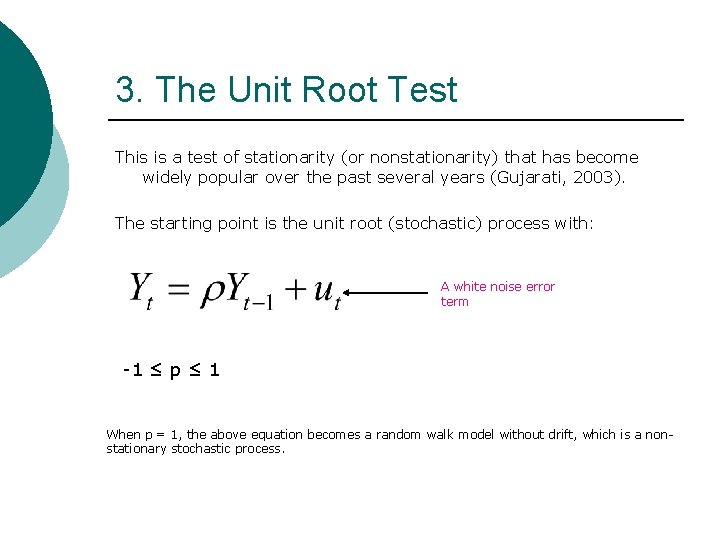
3. The Unit Root Test This is a test of stationarity (or nonstationarity) that has become widely popular over the past several years (Gujarati, 2003). The starting point is the unit root (stochastic) process with: A white noise error term -1 ≤ p ≤ 1 When p = 1, the above equation becomes a random walk model without drift, which is a nonstationary stochastic process.

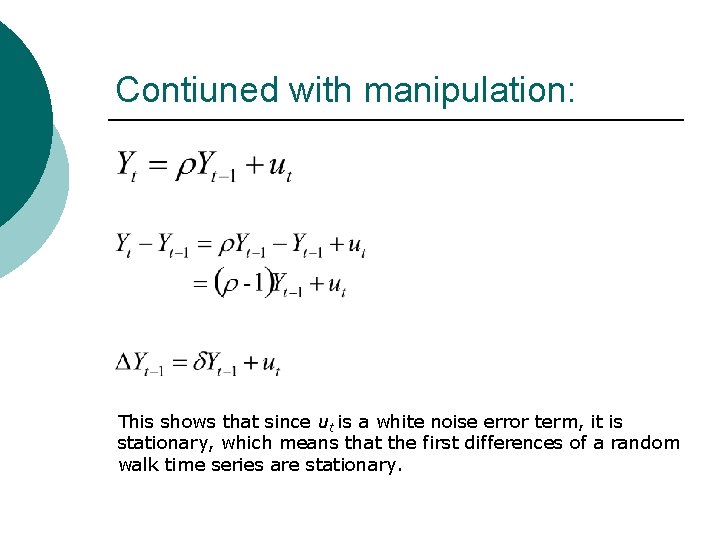
Contiuned with manipulation: This shows that since ut is a white noise error term, it is stationary, which means that the first differences of a random walk time series are stationary.

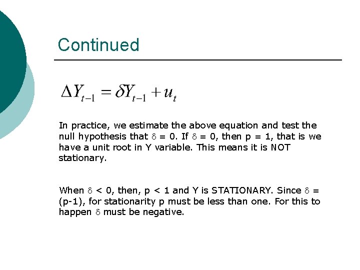
Continued In practice, we estimate the above equation and test the null hypothesis that = 0. If = 0, then p = 1, that is we have a unit root in Y variable. This means it is NOT stationary. When < 0, then, p < 1 and Y is STATIONARY. Since = (p-1), for stationarity p must be less than one. For this to happen must be negative.

Question: Which test to use for Unit Root? ¡ ¡ The estimated t value of Yt-1 does follow the t distribution even in large samples: It does not have an symptotic normal distribution. So? What is the alternative?

a. Dickey-Fuller (DF) Test (1979) ¡ DF has shown that under the null hypothesis that =0, the estimated t value of the coefficient of Yt-1 follows the (tau) statistic. ¡ DF have computed the critical values of statistic on the basis of Monte Carlo simulations. ¡ In the literature tau test is known as the DF test.

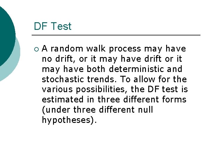
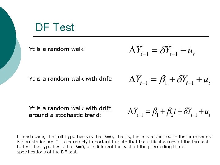
DF Test ¡ A random walk process may have no drift, or it may have drift or it may have both deterministic and stochastic trends. To allow for the various possibilities, the DF test is estimated in three different forms (under three different null hypotheses).

DF Test Yt is a random walk: Yt is a random walk with drift around a stochastic trend: In each case, the null hypothesis is that =0; that is, there is a unit root – the time series is non-stationary. It is extremely important to note that the critical values of the tau test to test the hypothesis that =0, are different for each of the preceeding three specifications of the DF test.

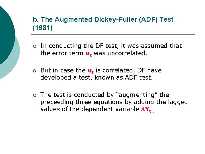
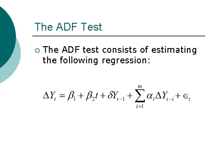
b. The Augmented Dickey-Fuller (ADF) Test (1981) ¡ In conducting the DF test, it was assumed that the error term ut was uncorrelated. ¡ But in case the ut is correlated, DF have developed a test, known as ADF test. ¡ The test is conducted by “augmenting” the preceeding three equations by adding the lagged values of the dependent variable Yt.

The ADF Test ¡ The ADF test consists of estimating the following regression:

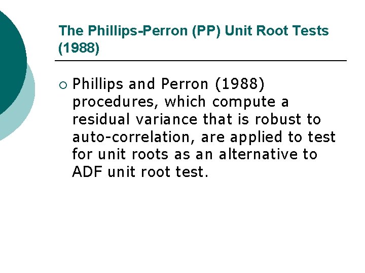
The Phillips-Perron (PP) Unit Root Tests (1988) ¡ Phillips and Perron (1988) procedures, which compute a residual variance that is robust to auto-correlation, are applied to test for unit roots as an alternative to ADF unit root test.

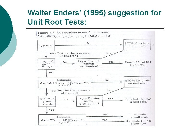
Walter Enders’ (1995) suggestion for Unit Root Tests:

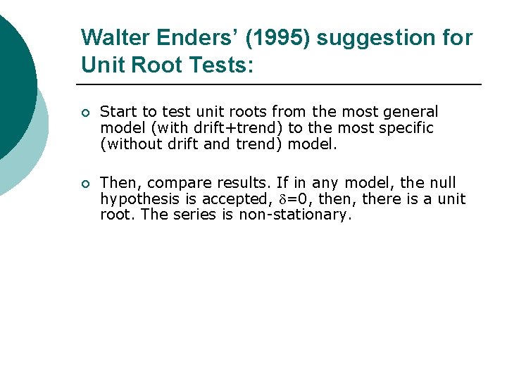
Walter Enders’ (1995) suggestion for Unit Root Tests: ¡ Start to test unit roots from the most general model (with drift+trend) to the most specific (without drift and trend) model. ¡ Then, compare results. If in any model, the null hypothesis is accepted, =0, then, there is a unit root. The series is non-stationary.

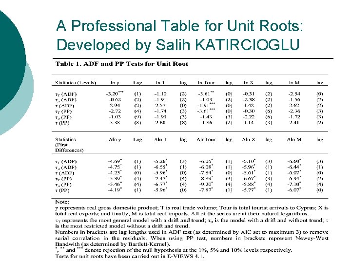
A Professional Table for Unit Roots: Developed by Salih KATIRCIOGLU

The Question is: ¡ There must be a lag level for testing unit roots. So, which lag level to select in running unit root tests? ¡ Two popular tests: Akaike Information Criterion (AIC) and Schwartz Information Criterion (SIC). ¡ These lag tests will be introduce in the application session. ¡ EVIEWS 5. 1 does these tests automatically.

Power of Test ¡ Most tests of the DF type have low power; that is, they tend to accept the null of unit root more frequently than is warranted. That is, these tests may find a unit root even when none exists. ¡ There are some reasons for low power, please refer to Gujarati (2003): p. 819.

c. KPSS Test for Unit Root ¡ To confirm the test results obtained from the ADF and PP tests, Kwiatkowski Phillips, Schmidt and Shin’s test (1992) (KPSS) is suggested to eliminate a possible low power against stationary near unit root processes which occurs in the ADF and PP tests. ¡ The KPSS test complements the ADF and PP tests in which the null hypothesis of KPSS test is that a series is stationary. This means that a stationary series is likely to have insignificant KPSS statistics and significant ADF and PP statistics.

Now is the Application Time of Unit Root Tests