Streaming Algorithms CS 6234 Advanced Algorithms February 10

Streaming Algorithms CS 6234 Advanced Algorithms February 10 2015 1

The stream model • Data sequentially enters at a rapid rate from one or more inputs • We cannot store the entire stream • Processing in real-time • Limited memory (usually sub linear in the size of the stream) • Goal: Compute a function of stream, e. g. , median, number of distinct elements, longest increasing sequence Approximate answer is usually preferable 2

Overview Counting bits with DGIM algorithm Bloom Filter Count-Min Sketch Approximate Heavy Hitters AMS Sketch Applications 3

Counting bits with DGIM algorithm Presented by Dmitrii Kharkovskii 4

Sliding windows • A useful model : queries are about a window of length N • The N most recent elements received (or last N time units) • Interesting case: N is still so large that it cannot be stored • Or, there are so many streams that windows for all cannot be stored 5

Problem description • Problem • Given a stream of 0’s and 1’s • Answer queries of the form “how many 1’s in the last k bits? ” where k ≤ N • Obvious solution • Store the most recent N bits (i. e. , window size = N) • When a new bit arrives, discard the N +1 st bit • Real Problem • Slow ‐ need to scan k‐bits to count • What if we cannot afford to store N bits? • Estimate with an approximate answer 6

Datar-Gionis-Indyk-Motwani Algorithm (DGIM) 7

Main idea of the algorithm Represent the window as a set of exponentially growing non-overlapping buckets 8

Timestamps • Each bit in the stream has a timestamp - the position in the stream from the beginning. • Record timestamps modulo N (window size) - use o(log N) bits • Store the most recent timestamp to identify the position of any other bit in the window 9

Buckets 10

Representing the stream by buckets • The right end of a bucket is always a position with a 1. • Every position with a 1 is in some bucket. • Buckets do not overlap. • There are one or two buckets of any given size, up to some maximum size. • All sizes must be a power of 2. • Buckets cannot decrease in size as we move to the left (back in time). 11

Updating buckets when a new bit arrives • Drop the last bucket if it has no overlap with the window • If the current bit is zero, no changes are needed • If the current bit is one • Create a new bucket with it. Size = 1, timestamp = current time modulo N. • If there are 3 buckets of size 1, merge two oldest into one of size 2. • If there are 3 buckets of size 2, merge two oldest into one of size 4. • . . . 12

Example of updating process 13

Query Answering How many ones are in the most recent k bits? • Find all buckets overlapping with last k bits • Sum the sizes of all but the oldest one Ans = 1 + 2 + 4 + 8/2 = 24 • Add the half of the size of the oldest one k 14

Memory requirements 15

Performance guarantee 16

References J. Leskovic, A. Rajamaran, J. Ulmann. “Mining of Massive Datasets”. Cambridge University Press 18

Bloom Filter Presented by. Naheed Anjum Arafat 19

Motivation: The “Set Membership” Problem • x: An Element • S: A Set of elements (Finite) • Input: x, S • Output: Streaming Algorithm: • Limited Space/item • Limited Processing time/item • Approximate answer based on a summary/sketch of the data stream in the memory. • True (if x in S) • False (if x not in S) Solution: Binary Search on an array of size |S|. Runtime Complexity: O(log|S|) 20

Bloom Filter • F F F F F 0 1 2 3 4 5 6 7 8 9 n = 10 21

Bloom Filter • F TF F F FT F TF 0 1 2 3 4 5 6 F F F 7 8 9 k = 3 22

Bloom Filter • Note: A particular Boolean value may be set to True several times. F T F 0 1 2 3 4 5 T 6 TF F FT 7 8 9 k = 3 23

Algorithm to Approximate Set Membership Query Input: x ( may/may not be an element) Output: Boolean For all i ϵ {0, 1, …, k-1} if hi(x) is False return False return True Runtime Complexity: - O(k) F T F T 0 1 2 3 4 5 6 7 8 9 k = 3 24

Algorithm to Approximate Set Membership Query False Positive!! F T 0 1 F F T T F T 2 3 4 5 6 7 8 9 k = 3 25

Error Types • False Negative – Answering “is not there” on an element which “is there” • Never happens for Bloom Filter • False Positive – Answering “is there” for an element which “is not there” • Might happens. How likely? 26

Probability of false positives S 2 S 1 F T F T F n = size of table m = number of items k = number of hash functions 27

Probability of false positives S 1 F T S 2 F F T F n = size of table m = number of items k = number of hash functions 28

Probability of false positives S 1 F T S 2 F F T n = size of table m = number of items k = number of hash functions F T F Approximate Probability of False Positive For a fixed m, n which value of k will minimize this bound? Bit per item 29

Bloom Filters: cons • Small false positive probability • Cannot handle deletions • Size of the Bit vector has to be set a priori in order to maintain a predetermined FP-rates : - Resolved in “Scalable Bloom Filter” – Almeida, Paulo; Baquero, Carlos; Preguica, Nuno; Hutchison, David (2007), "Scalable Bloom Filters" (PDF), Information Processing Letters 101 (6): 255– 261 30

References • https: //en. wikipedia. org/wiki/Bloom_filter • Graham Cormode, Sketch Techniques for Approximate Query Processing, ATT Research • Michael Mitzenmacher, Compressed Bloom Filters, Harvard University, Cambridge 31

Count-Min Sketch Erick Purwanto A 0050717 L

Motivation Count-Min Sketch •

Frequency Query •

Count-Min Sketch •

Count-Min Sketch • CM

Collision •

Count-Min Sketch Analysis •

Count-Min Sketch •

Approximate Heavy Hitters Tae. Hoon Joseph, Kim

Count-Min Sketch (CMS) •

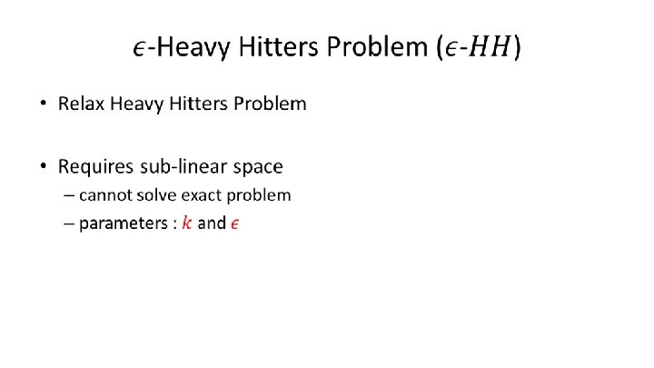
Heavy Hitters Problem •

Heavy Hitters Problem: Naïve Solution •

Naïve Solution using CMS … … m-2 m-1 m j …

Naïve Solution using CMS •

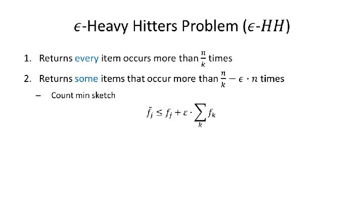
Better Solution •

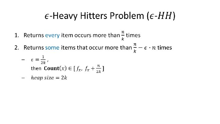
Algorithm Approximate Heavy Hitters •

EXAMPLES 1 Min-Heap 4 1 1 … 1

EXAMPLES 1 Min-Heap 4 {1: 4} 1 1 … 1

1 2 3 4 5 4 2 6 9 3 EXAMPLES Min-Heap {1: 3} {1: 2} {1: 9} {1: 4} 1 1 … 1 {1: 6}

1 2 3 4 5 6 4 2 6 9 3 4 EXAMPLES Min-Heap {1: 3} {1: 2} {1: 9} 1 {1: 4} 1 … 1 {1: 6}

1 2 3 4 5 6 4 2 6 9 3 4 EXAMPLES Min-Heap {1: 3} {1: 2} {1: 9} 2 {1: 4} 2 … 2 {1: 6}

1 2 3 4 5 6 4 2 6 9 3 4 EXAMPLES Min-Heap {2: 4} 2 2 … 2

EXAMPLES 79 … Min-Heap 2 {16: 4} {20: 9} 16 18 … 15 {23: 6}

EXAMPLES 79 … Min-Heap 2 {16: 4} {20: 9} 17 19 … 16 {23: 6}

EXAMPLES 79 … Min-Heap 2 {16: 2} {16: 4} {20: 9} 17 19 … 16 {23: 6}

… 79 80 81 2 EXAMPLES Min-Heap {16: 2} {16: 4} {20: 9} 3 6 … 4 {23: 6}

… 79 80 81 2 1 9 EXAMPLES Min-Heap {16: 2} {16: 4} {20: 9} 20 24 … 25 {23: 6}

… 79 80 81 2 1 9 EXAMPLES Min-Heap {16: 2} {16: 4} {20: 9} 21 25 … 26 {23: 6}

… 79 80 81 2 1 9 EXAMPLES Min-Heap {21: 9} {23: 6} 21 25 … 26

Analysis •

AMS Sketch : Estimate Second Moment Dissanayaka Mudiyanselage Emil Manupa Karunaratne

The Second Moment • Stream : • The Second Moment : • The trivial solution would be : maintain a histogram of size n and get the sum of squares • Its not feasible maintain that large array, therefore we intend to find a approximation algorithm to achieve sub-linear space complexity with bounded errors • The algorithm will give an estimate within ε relative error with δ failure probability. (Two Parameters)

The Method • j is the next item in the stream. • 2 -wise independent d hash functions to find the bucket for each row • After finding the bucket, 4 -wise independent d hash functions to decide inc/dec : • In a summary :

The Method •

Why should this method give F 2 ? • For kth row : • Estimate F 2 from kth row : • Each row there would be : • First part : • Second part : g(i)g(j) can be +1 or -1 with equal probability, therefore the expectation is 0.

What guarantee can we give about the accuracy ? •

Space and Time Complexity •

AMS Sketch and Applications Sapumal Ahangama

Hash functions •

Hash functions • These hash functions can be computed very quickly, faster even than more familiar (cryptographic) hash functions • For scenarios which require very high throughput, efficient implementations are available for hash functions, – Based on optimizations for particular values of p, and partial precomputations – Ref: M. Thorup and Y. Zhang. Tabulation based 4 -universal hashing with applications to second moment estimation. In ACM-SIAM Symposium on Discrete Algorithms, 2004

Time complexity - Update •

Time complexity - Query •

Applications - Inner product •

Inner Product •

Inner Product – Join size estimation • Inner product has a natural interpretation, as the size of the equi-join between two relations… • In SQL, SELECT COUNT(*) FROM D, D’ WHERE D. id = D’. id

Example UPDATE(23, 1) 23 h 1 d = 3 h 2 h 3 1 2 3 4 5 6 7 8 1 0 0 0 0 2 0 0 0 0 3 0 0 0 0 w=8 87

Example UPDATE(23, 1) 23 h 1 h 2 d = 3 h 3 1 2 3 4 5 6 7 8 1 0 0 -1 0 0 0 2 -1 0 0 0 0 3 0 0 0 +1 0 w=8 88

Example UPDATE(99, 2) 99 h 1 d = 3 h 2 h 3 1 2 3 4 5 6 7 8 1 0 0 -1 0 0 0 2 -1 0 0 0 0 3 0 0 0 +1 0 w=8 89

Example UPDATE(99, 2) 99 h 1 h 2 d = 3 h 3 1 2 3 4 5 6 7 8 1 0 0 -1 0 0 0 2 -1 0 0 0 0 3 0 0 0 +1 0 w=8 90

Example UPDATE(99, 2) 99 h 1 h 2 d = 3 h 3 1 2 3 4 5 6 7 8 1 0 0 -1 0 +2 0 0 0 2 -3 0 0 0 0 3 0 0 +2 0 0 0 +1 0 w=8 91