High Frequency Trading Strategies MSE 444 Paul Merolla

High Frequency Trading Strategies MS&E 444 Paul Merolla Erik Anderson Alexis Pribula

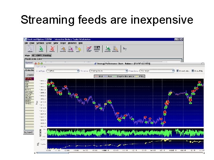
Streaming feeds are inexpensive

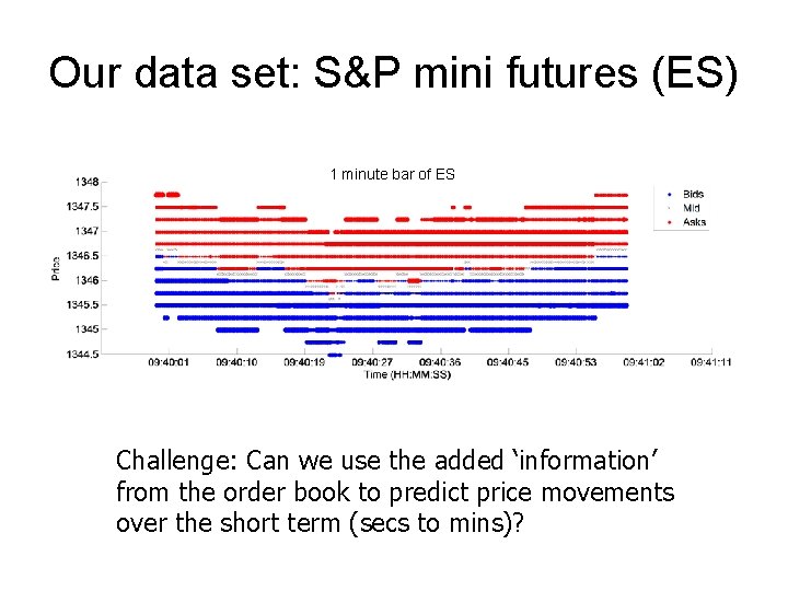
Our data set: S&P mini futures (ES) 1 minute bar of ES Challenge: Can we use the added ‘information’ from the order book to predict price movements over the short term (secs to mins)?

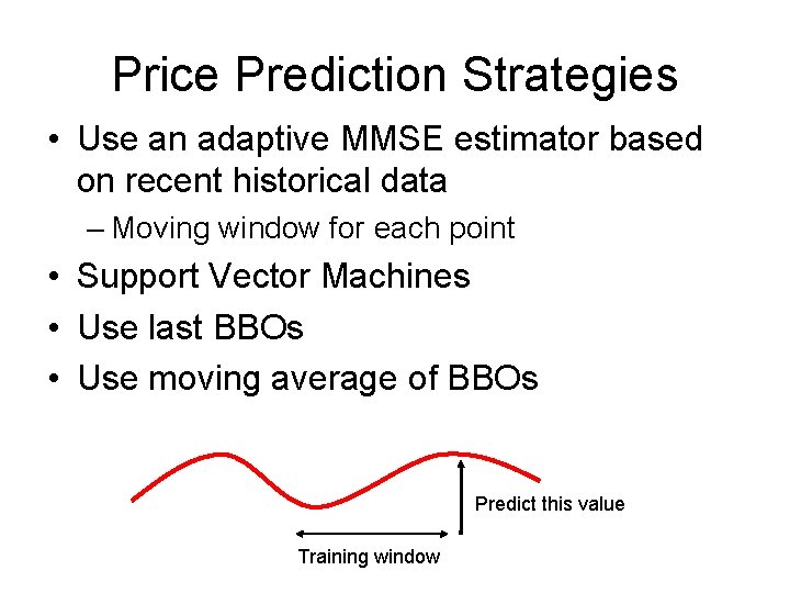
Price Prediction Strategies • Use an adaptive MMSE estimator based on recent historical data – Moving window for each point • Support Vector Machines • Use last BBOs • Use moving average of BBOs Predict this value Training window

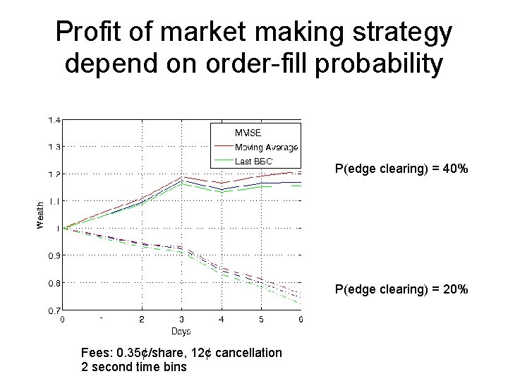
Profit of market making strategy depend on order-fill probability P(edge clearing) = 40% P(edge clearing) = 20% Fees: 0. 35¢/share, 12¢ cancellation 2 second time bins

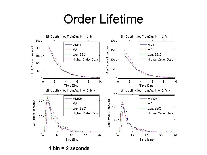
Order Lifetime 1 bin = 2 seconds

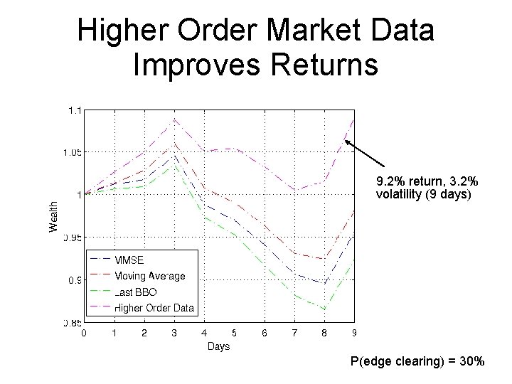
Higher Order Market Data Improves Returns 9. 2% return, 3. 2% volatility (9 days) P(edge clearing) = 30%

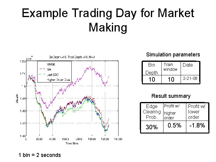
Example Trading Day for Market Making Simulation parameters Bin Depth 10 Train window 10 Date 2 -21 -08 Result summary Edge Profit w/ Clearing higher Prob. order Time Bin 1 bin = 2 seconds 30% 0. 5% Profit w/ lower order -1. 8%

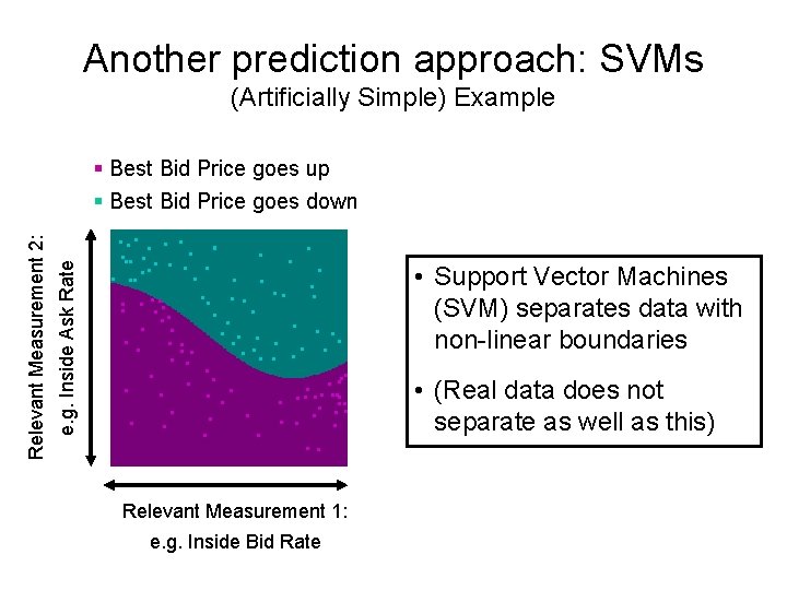
Another prediction approach: SVMs (Artificially Simple) Example e. g. Inside Ask Rate Relevant Measurement 2: Best Bid Price goes up Best Bid Price goes down • Support Vector Machines (SVM) separates data with non-linear boundaries • (Real data does not separate as well as this) Relevant Measurement 1: e. g. Inside Bid Rate

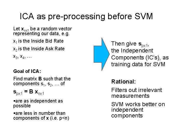
ICA as pre-processing before SVM Let xnx 1 be a random vector representing our data, e. g. x 1 is the Inside Bid Rate x 2 is the Inside Ask Rate x 3, x 4, … Then give spx 1, the Independent Components (IC’s), as training data for SVM Goal of ICA: Find matrix B such that the components s 1, s 2, … of spx 1 = B xnx 1 are as independent as possible are less in number than components of x (i. e. p<n) Rational: Filters out irrelevant measurements SVM works better on independent components

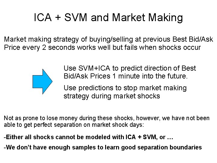
ICA + SVM and Market Making Market making strategy of buying/selling at previous Best Bid/Ask Price every 2 seconds works well but fails when shocks occur Use SVM+ICA to predict direction of Best Bid/Ask Prices 1 minute into the future. Use predictions to stop market making strategy during market shocks Not as prone to lose money during these shocks, however, we have not been able to get perfect separation on market shock days: -Either all shocks cannot be modeled with ICA + SVM, or … -We don’t have enough samples to learn good separation boundaries

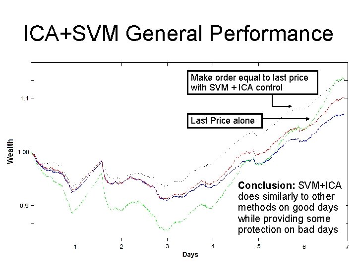
ICA+SVM General Performance Make order equal to last price with SVM + ICA control Last Price alone Conclusion: SVM+ICA does similarly to other methods on good days while providing some protection on bad days