Quantum Computing Lecture 1 Introduction and Quantum Theory

Quantum Computing Lecture 1: Introduction and Quantum Theory Dave Bacon Department of Computer Science & Engineering University of Washington

Quantum Computing Professor Mark Oskin (University of Washington, CS&E) 1. Sunk his boat. 2. Salvaged (recovered) his boat. 3. Dropped his boat on his foot. 4. Bad for Mark, but good for me! Slides also available at http: //www. cs. washington. edu/homes/dabacon/teaching/siena

Warning! Two foreign languages for the price of one speaker: English and Quantum Theory Do not be shy! Please, ask me to repeat, to rephrase, or to just plain slow down.

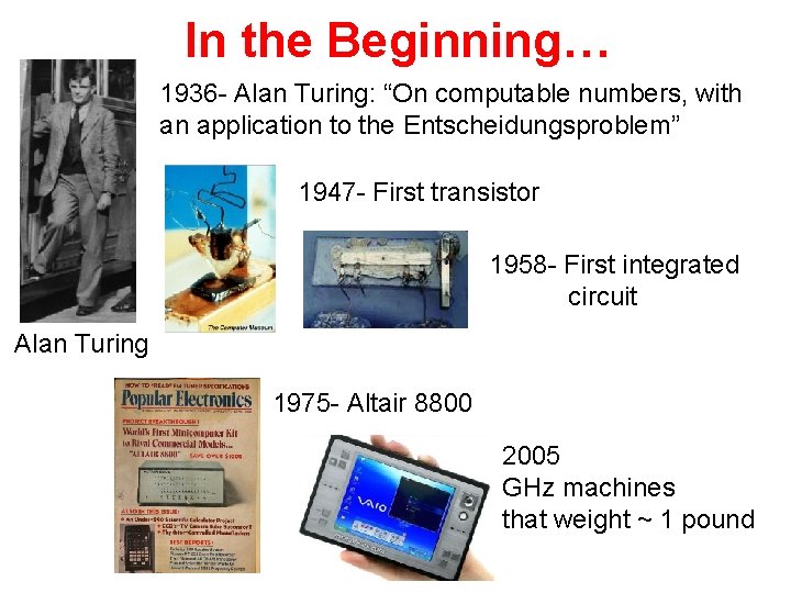
In the Beginning… 1936 - Alan Turing: “On computable numbers, with an application to the Entscheidungsproblem” 1947 - First transistor 1958 - First integrated circuit Alan Turing 1975 - Altair 8800 2005 GHz machines that weight ~ 1 pound

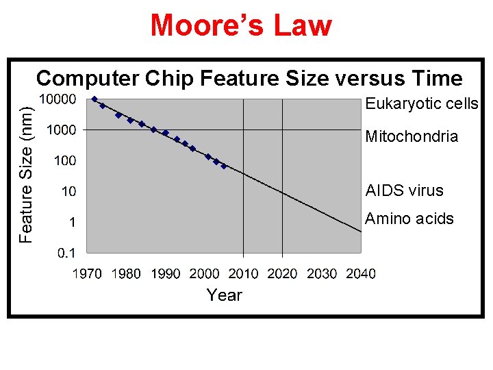
Moore’s Law Computer Chip Feature Size versus Time Eukaryotic cells Mitochondria AIDS virus Amino acids

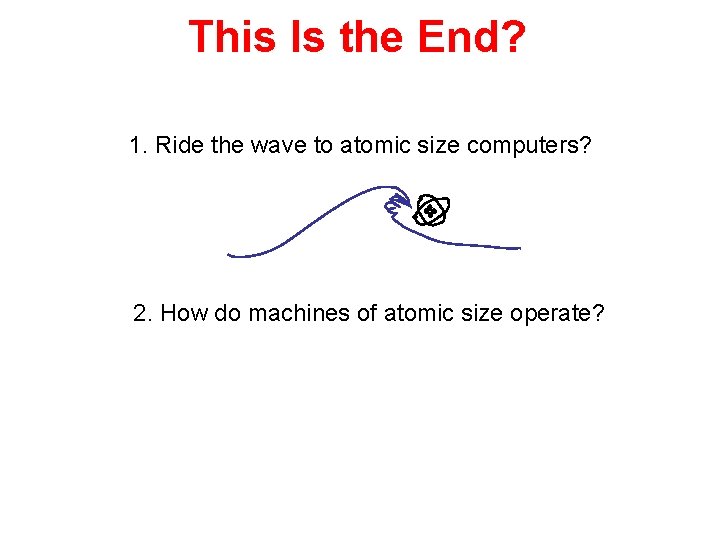
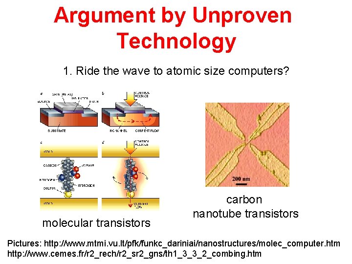
This Is the End? 1. Ride the wave to atomic size computers? 2. How do machines of atomic size operate?

Argument by Unproven Technology 1. Ride the wave to atomic size computers? molecular transistors carbon nanotube transistors Pictures: http: //www. mtmi. vu. lt/pfk/funkc_dariniai/nanostructures/molec_computer. htm http: //www. cemes. fr/r 2_rech/r 2_sr 2_gns/th 1_3_3_2_combing. htm

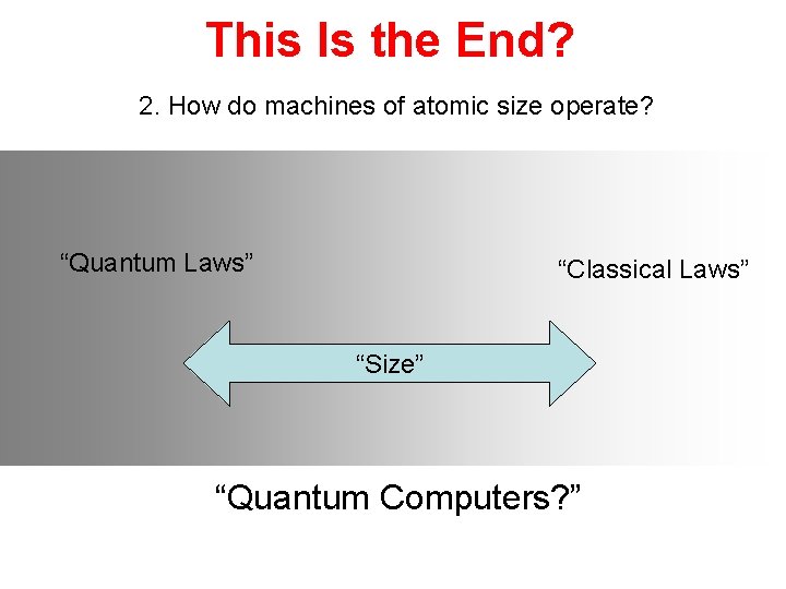
This Is the End? 2. How do machines of atomic size operate? “Quantum Laws” “Classical Laws” “Size” “Quantum Computers? ”

This Is the End? 2. How do machines of atomic size operate? Richard Feynman David Deutsch Paul Benioff

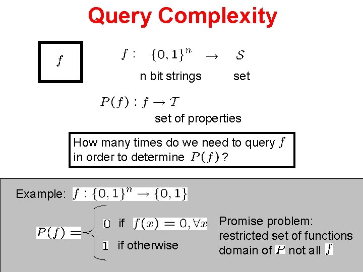
Query Complexity n bit strings set of properties How many times do we need to query in order to determine ? Example: if if otherwise Promise problem: restricted set of functions domain of not all

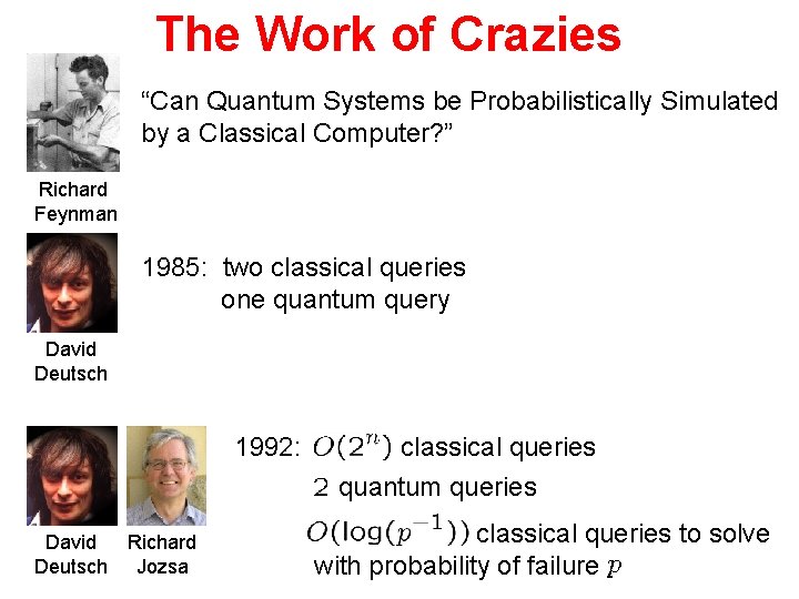
The Work of Crazies “Can Quantum Systems be Probabilistically Simulated by a Classical Computer? ” Richard Feynman 1985: two classical queries one quantum query David Deutsch 1992: David Richard Deutsch Jozsa classical queries quantum queries classical queries to solve with probability of failure

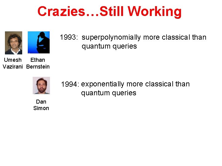
Crazies…Still Working 1993: superpolynomially more classical than quantum queries Umesh Ethan Vazirani Bernstein 1994: exponentially more classical than quantum queries Dan Simon

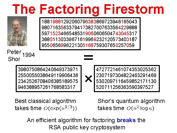
The Factoring Firestorm 18819881292060796383869723946165043 98071635633794173827007633564229888 59715234665485319060606504743045317 38801130339671619969232120573403187 9550656996221305168759307650257059 Peter 1994 Shor 3980750864240649373971 2550055038649119906436 2342526708406385189575 946388957261768583317 Best classical algorithm takes time 4727721461074353025362 2307197304822463291469 5302097116459852171130 520711256363590397527 Shor’s quantum algorithm takes time An efficient algorithm for factoring breaks the RSA public key cryptosystem

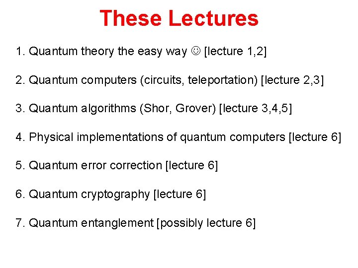
These Lectures 1. Quantum theory the easy way [lecture 1, 2] 2. Quantum computers (circuits, teleportation) [lecture 2, 3] 3. Quantum algorithms (Shor, Grover) [lecture 3, 4, 5] 4. Physical implementations of quantum computers [lecture 6] 5. Quantum error correction [lecture 6] 6. Quantum cryptography [lecture 6] 7. Quantum entanglement [possibly lecture 6]

Quantum Theory “The Easy Way”

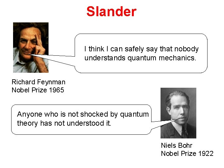
Slander I think I can safely say that nobody understands quantum mechanics. Richard Feynman Nobel Prize 1965 Anyone who is not shocked by quantum theory has not understood it. Niels Bohr Nobel Prize 1922

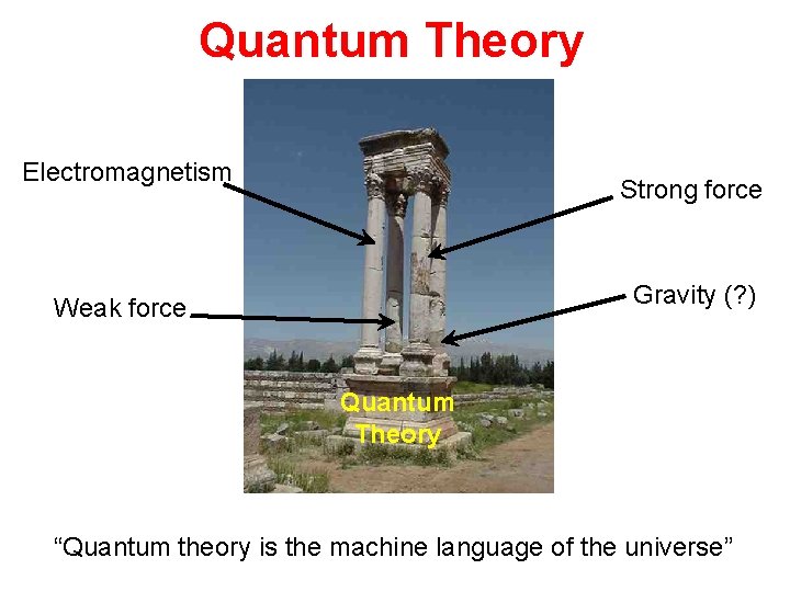
Quantum Theory Electromagnetism Strong force Gravity (? ) Weak force Quantum Theory “Quantum theory is the machine language of the universe”

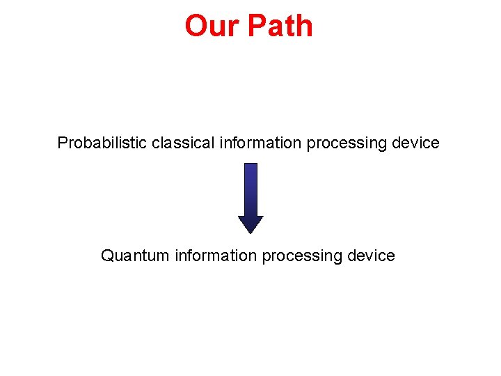
Our Path Probabilistic classical information processing device Quantum information processing device

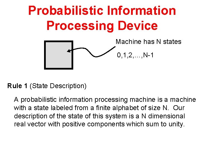
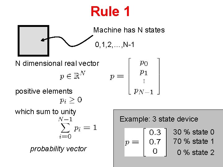
Probabilistic Information Processing Device Machine has N states 0, 1, 2, …, N-1 Rule 1 (State Description) A probabilistic information processing machine is a machine with a state labeled from a finite alphabet of size N. Our description of the state of this system is a N dimensional real vector with positive components which sum to unity.

Rule 1 Machine has N states 0, 1, 2, …, N-1 N dimensional real vector positive elements which sum to unity probability vector Example: 3 state device 30 % state 0 70 % state 1 0 % state 2

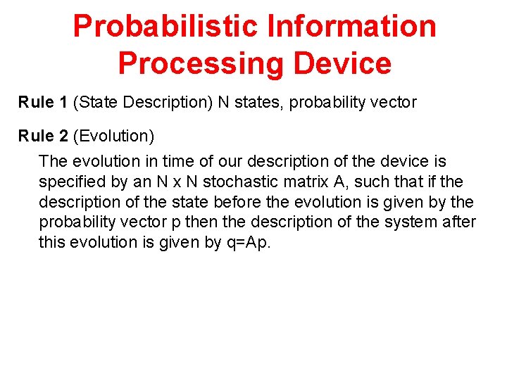
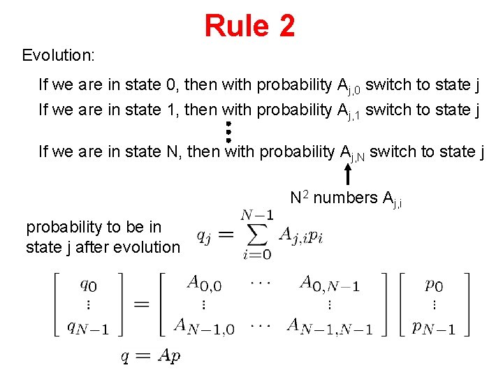
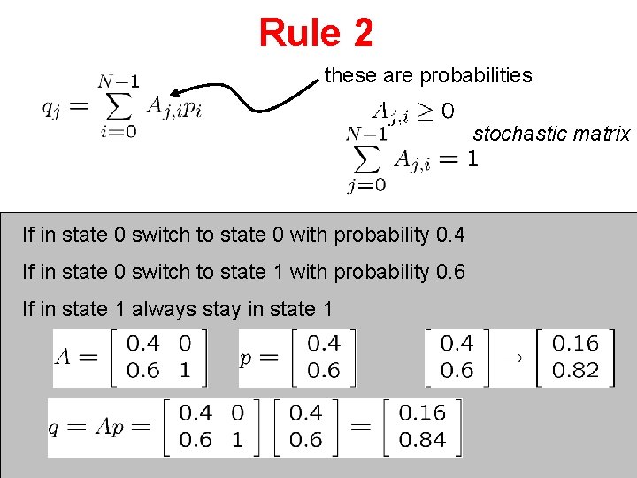
Probabilistic Information Processing Device Rule 1 (State Description) N states, probability vector Rule 2 (Evolution) The evolution in time of our description of the device is specified by an N x N stochastic matrix A, such that if the description of the state before the evolution is given by the probability vector p then the description of the system after this evolution is given by q=Ap.

Rule 2 Evolution: If we are in state 0, then with probability Aj, 0 switch to state j If we are in state 1, then with probability Aj, 1 switch to state j If we are in state N, then with probability Aj, N switch to state j N 2 numbers Aj, i probability to be in state j after evolution

Rule 2 these are probabilities stochastic matrix If in state 0 switch to state 0 with probability 0. 4 If in state 0 switch to state 1 with probability 0. 6 If in state 1 always stay in state 1

Probabilistic Information Processing Device Rule 1 (State Description) N states, probability vector Rule 2 (Evolution) N x N stochastic matrix Rule 3 (Measurement) A measurement in the computational basis of our N dimensional system which is described by a probability vector p yields outcome j given by the jth component of p. After the measurement, the system is described by a probability vector with certainty that the state is j.

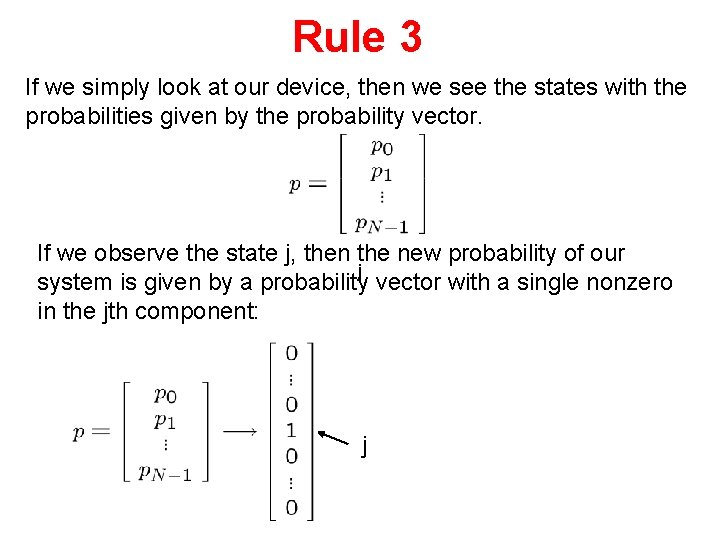
Rule 3 If we simply look at our device, then we see the states with the probabilities given by the probability vector. If we observe the state j, then the new probability of our j system is given by a probability vector with a single nonzero in the jth component: j

Probabilistic Information Processing Device Rule 1 (State Description) N states, probability vector Rule 2 (Evolution) N x N stochastic matrix Rule 3 (Measurement) k conditional probability vectors Rule 4 (Composite Systems) Two devices can be combined to form a bigger device. If these devices have N and M states, respectively, then the composite system has NM states. The probability vector for this new machine is a real NM dimensional probability vector from.

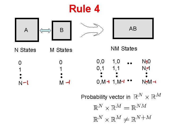
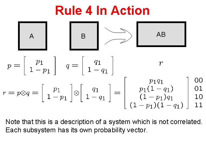
Rule 4 A B N States M States AB NM States 0 1 0, 0 0, 1 1, 0 1, 1 N, 0 N, 1 N M 0, M 1, M N, M Probability vector in

Rule 4 In Action A B AB Note that this is a description of a system which is not correlated. Each subsystem has its own probability vector.

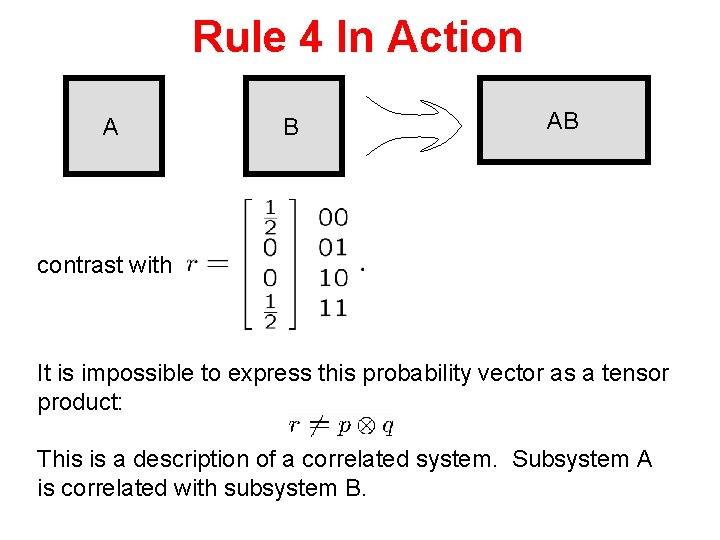
Rule 4 In Action A B AB contrast with It is impossible to express this probability vector as a tensor product: This is a description of a correlated system. Subsystem A is correlated with subsystem B.

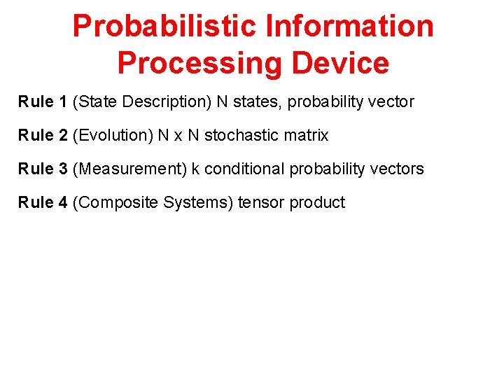
Probabilistic Information Processing Device Rule 1 (State Description) N states, probability vector Rule 2 (Evolution) N x N stochastic matrix Rule 3 (Measurement) k conditional probability vectors Rule 4 (Composite Systems) tensor product

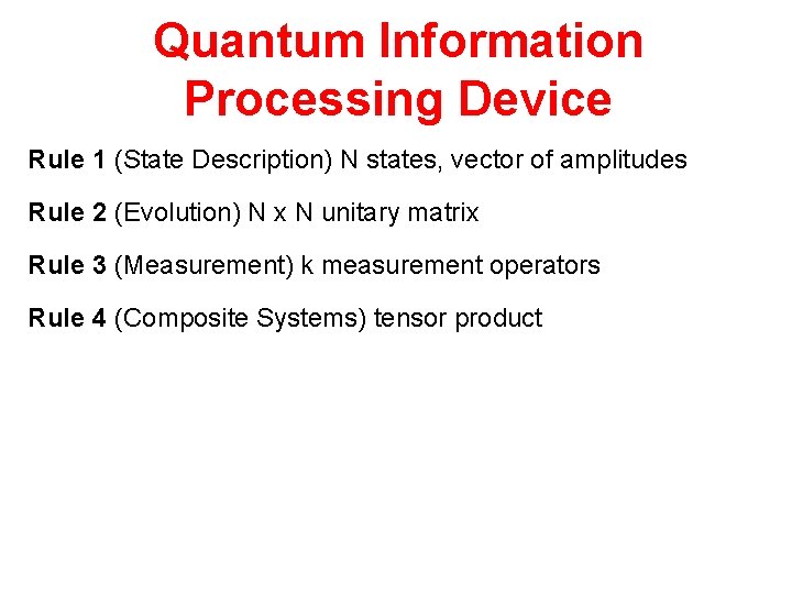
Quantum Information Processing Device Rule 1 (State Description) N states, vector of amplitudes Rule 2 (Evolution) N x N unitary matrix Rule 3 (Measurement) k measurement operators Rule 4 (Composite Systems) tensor product

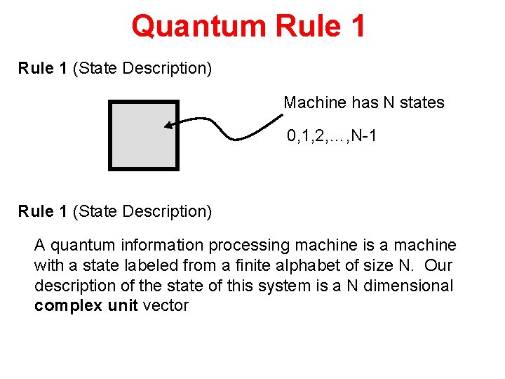
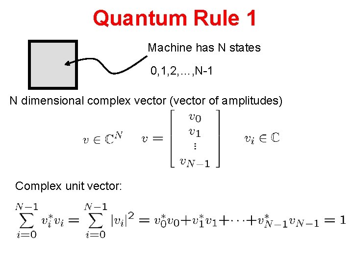
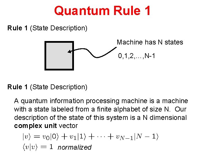
Quantum Rule 1 (State Description) Machine has N states 0, 1, 2, …, N-1 Rule 1 (State Description) A quantum information processing machine is a machine with a state labeled from a finite alphabet of size N. Our description of the state of this system is a N dimensional complex unit vector

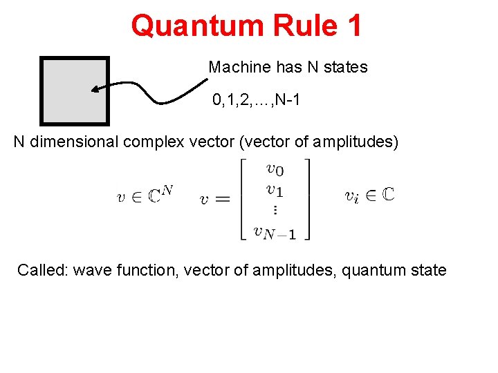
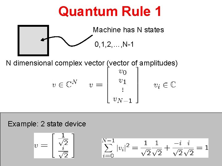
Quantum Rule 1 Machine has N states 0, 1, 2, …, N-1 N dimensional complex vector (vector of amplitudes) Called: wave function, vector of amplitudes, quantum state

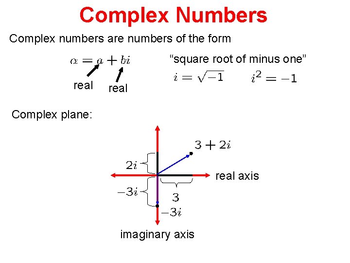
Complex Numbers Complex numbers are numbers of the form “square root of minus one” real Complex plane: real axis imaginary axis

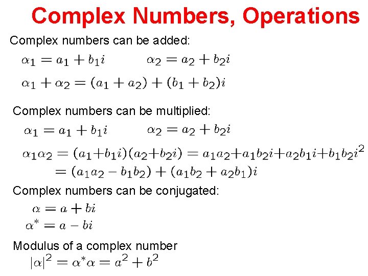
Complex Numbers, Operations Complex numbers can be added: Complex numbers can be multiplied: Complex numbers can be conjugated: Modulus of a complex number

Quantum Rule 1 Machine has N states 0, 1, 2, …, N-1 N dimensional complex vector (vector of amplitudes) Complex unit vector:

Quantum Rule 1 Machine has N states 0, 1, 2, …, N-1 N dimensional complex vector (vector of amplitudes) Example: 2 state device

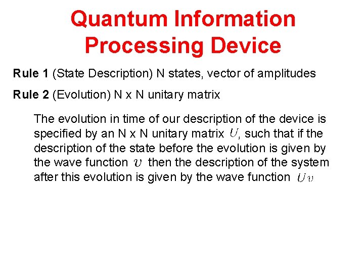
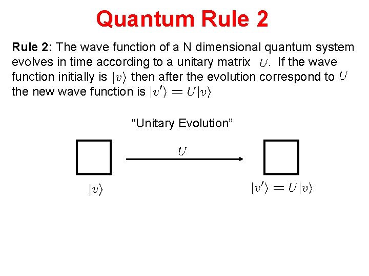
Quantum Information Processing Device Rule 1 (State Description) N states, vector of amplitudes Rule 2 (Evolution) N x N unitary matrix The evolution in time of our description of the device is specified by an N x N unitary matrix , such that if the description of the state before the evolution is given by the wave function the description of the system after this evolution is given by the wave function

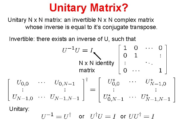
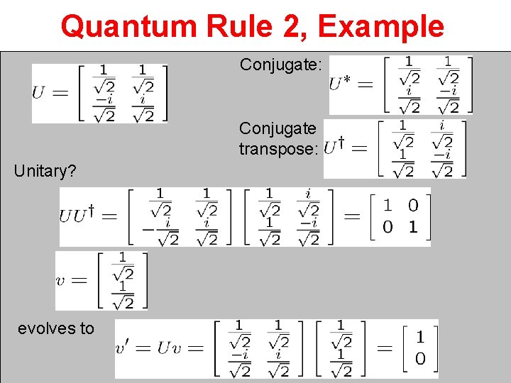
Unitary Matrix? Unitary N x N matrix: an invertible N x N complex matrix whose inverse is equal to it’s conjugate transpose. Invertible: there exists an inverse of U, such that N x N identity matrix Unitary: or or

Quantum Rule 2, Example Conjugate: Conjugate transpose: Unitary? evolves to

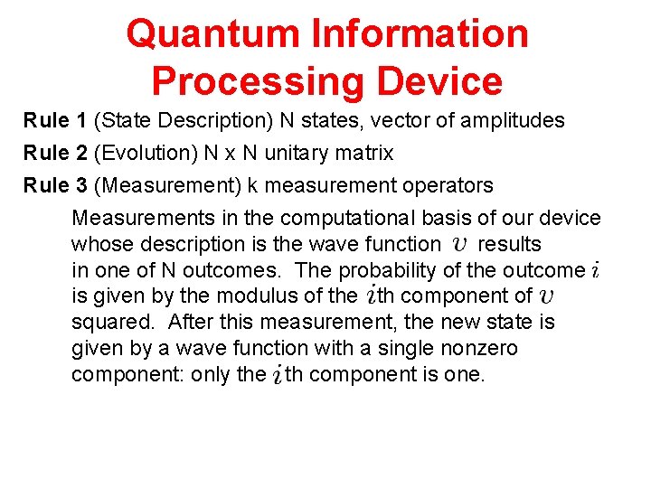
Quantum Information Processing Device Rule 1 (State Description) N states, vector of amplitudes Rule 2 (Evolution) N x N unitary matrix Rule 3 (Measurement) k measurement operators Measurements in the computational basis of our device whose description is the wave function results in one of N outcomes. The probability of the outcome is given by the modulus of the th component of squared. After this measurement, the new state is given by a wave function with a single nonzero component: only the th component is one.

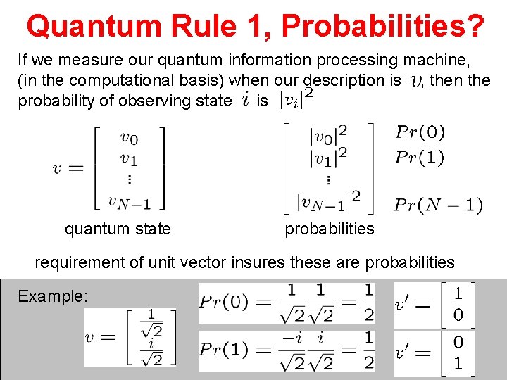
Quantum Rule 1, Probabilities? If we measure our quantum information processing machine, (in the computational basis) when our description is , then the probability of observing state is. quantum state probabilities requirement of unit vector insures these are probabilities Example:

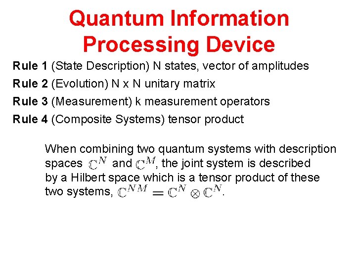
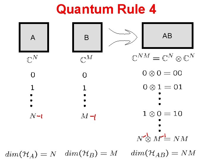
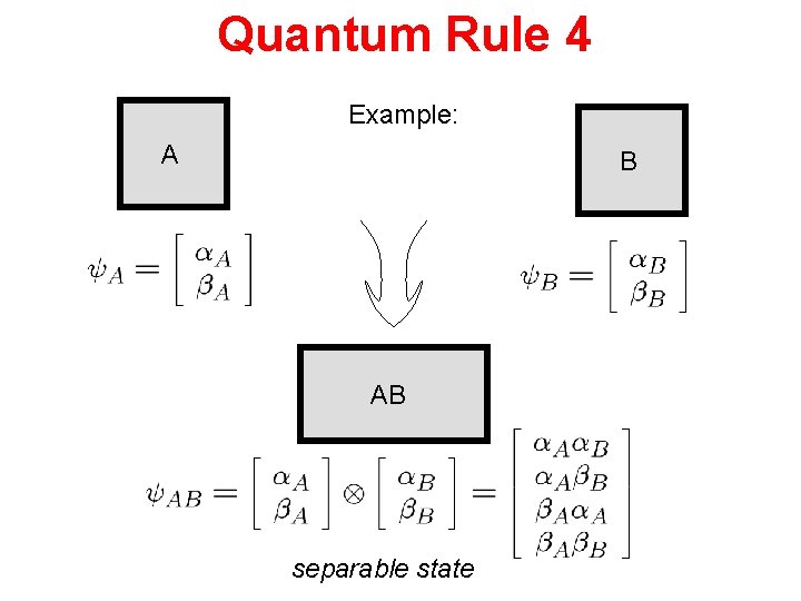
Quantum Information Processing Device Rule 1 (State Description) N states, vector of amplitudes Rule 2 (Evolution) N x N unitary matrix Rule 3 (Measurement) k measurement operators Rule 4 (Composite Systems) tensor product When combining two quantum systems with description spaces and , the joint system is described by a Hilbert space which is a tensor product of these two systems, .

Quantum Rule 4 A B AB

Quantum Rule 4 Example: A B AB separable state

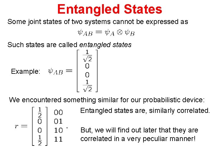
Entangled States Some joint states of two systems cannot be expressed as Such states are called entangled states Example: We encountered something similar for our probabilistic device: Entangled states are, similarly correlated. But, we will find out later that they are correlated in a very peculiar manner!

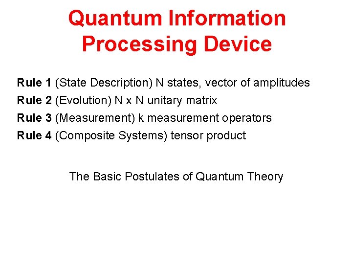
Quantum Information Processing Device Rule 1 (State Description) N states, vector of amplitudes Rule 2 (Evolution) N x N unitary matrix Rule 3 (Measurement) k measurement operators Rule 4 (Composite Systems) tensor product The Basic Postulates of Quantum Theory

These are the Laws We need to learn notation, and all about quantum circuits.

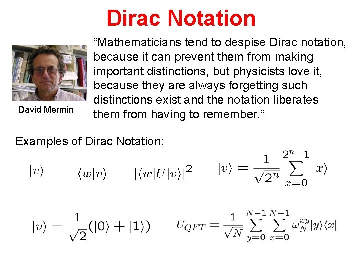
Dirac Notation David Mermin “Mathematicians tend to despise Dirac notation, because it can prevent them from making important distinctions, but physicists love it, because they are always forgetting such distinctions exist and the notation liberates them from having to remember. ” Examples of Dirac Notation:

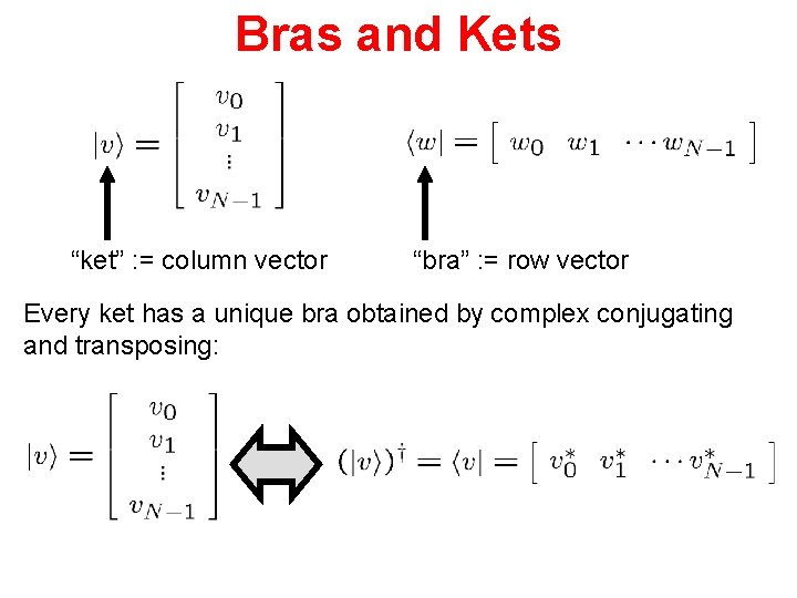
Bras and Kets “ket” : = column vector “bra” : = row vector Every ket has a unique bra obtained by complex conjugating and transposing:

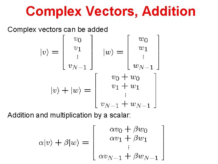
Complex Vectors, Addition Complex vectors can be added Addition and multiplication by a scalar:

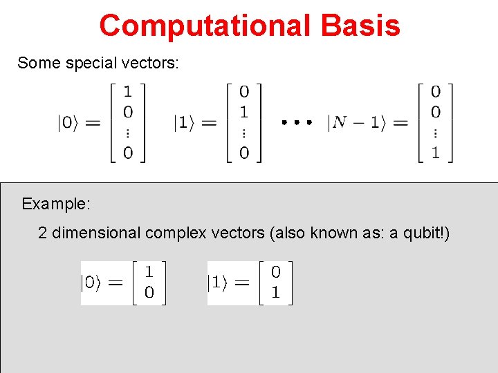
Computational Basis Some special vectors: Example: 2 dimensional complex vectors (also known as: a qubit!)

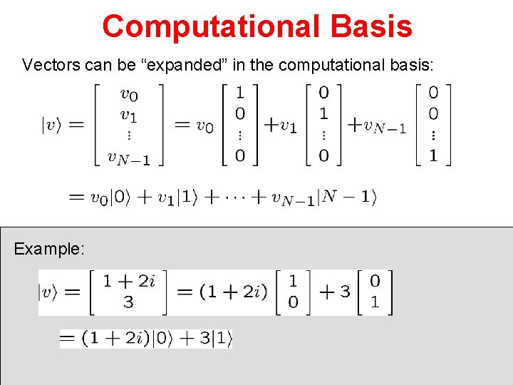
Computational Basis Vectors can be “expanded” in the computational basis: Example:

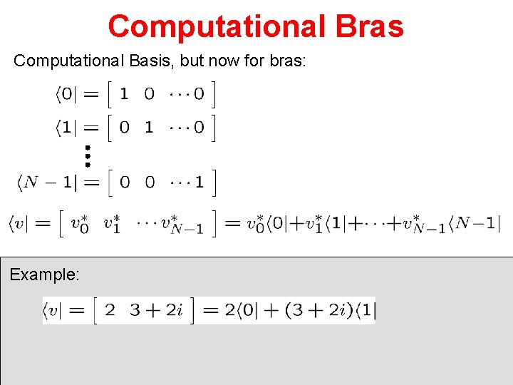
Computational Bras Computational Basis, but now for bras: Example:

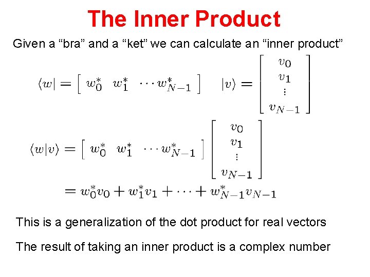
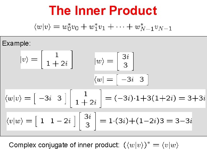
The Inner Product Given a “bra” and a “ket” we can calculate an “inner product” This is a generalization of the dot product for real vectors The result of taking an inner product is a complex number

The Inner Product Example: Complex conjugate of inner product:

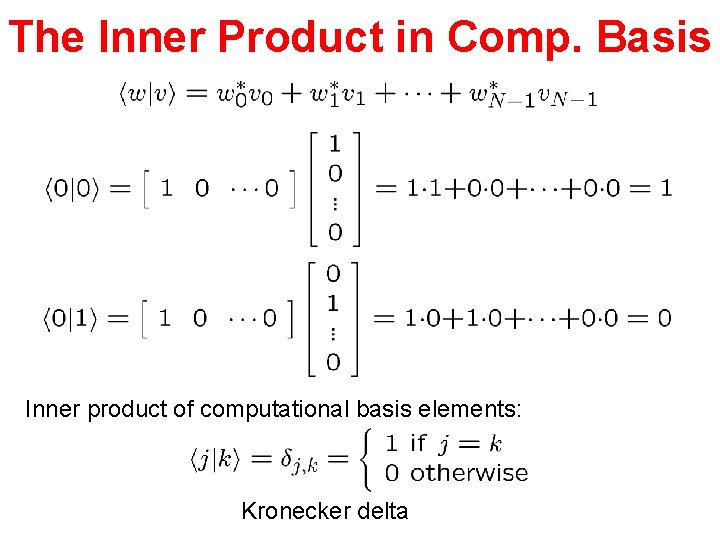
The Inner Product in Comp. Basis Inner product of computational basis elements: Kronecker delta

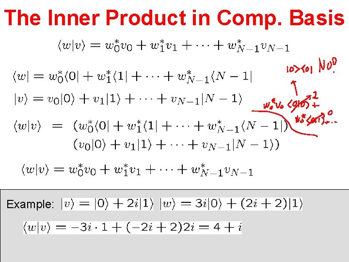
The Inner Product in Comp. Basis Example:

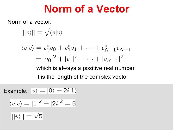
Norm of a Vector Norm of a vector: which is always a positive real number it is the length of the complex vector Example:

Quantum Rule 1 (State Description) Machine has N states 0, 1, 2, …, N-1 Rule 1 (State Description) A quantum information processing machine is a machine with a state labeled from a finite alphabet of size N. Our description of the state of this system is a N dimensional complex unit vector normalized

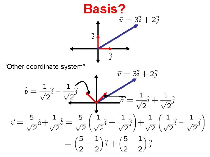
Basis? “Other coordinate system”

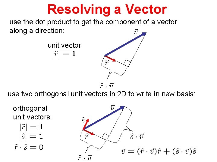
Resolving a Vector use the dot product to get the component of a vector along a direction: unit vector use two orthogonal unit vectors in 2 D to write in new basis: orthogonal unit vectors:

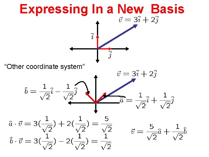
Expressing In a New Basis “Other coordinate system”

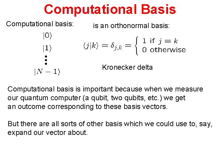
Computational Basis Computational basis: is an orthonormal basis: Kronecker delta Computational basis is important because when we measure our quantum computer (a qubit, two qubits, etc. ) we get an outcome corresponding to these basis vectors. But there all sorts of other basis which we could use to, say, expand our vector about.

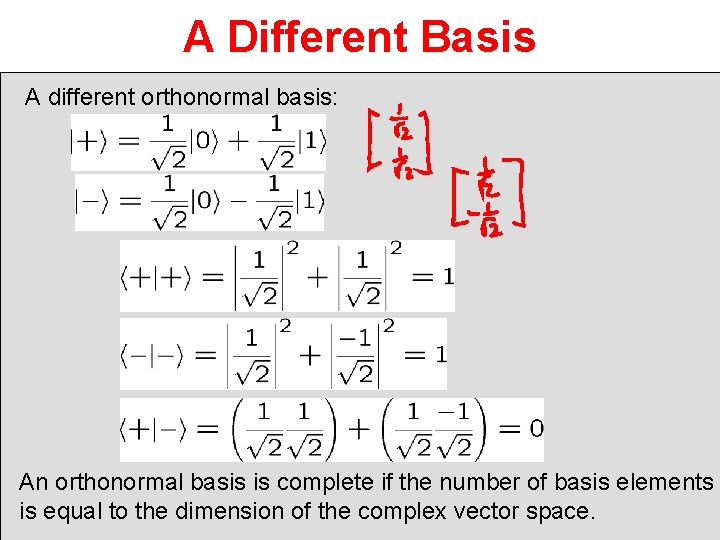
A Different Basis A different orthonormal basis: An orthonormal basis is complete if the number of basis elements is equal to the dimension of the complex vector space.

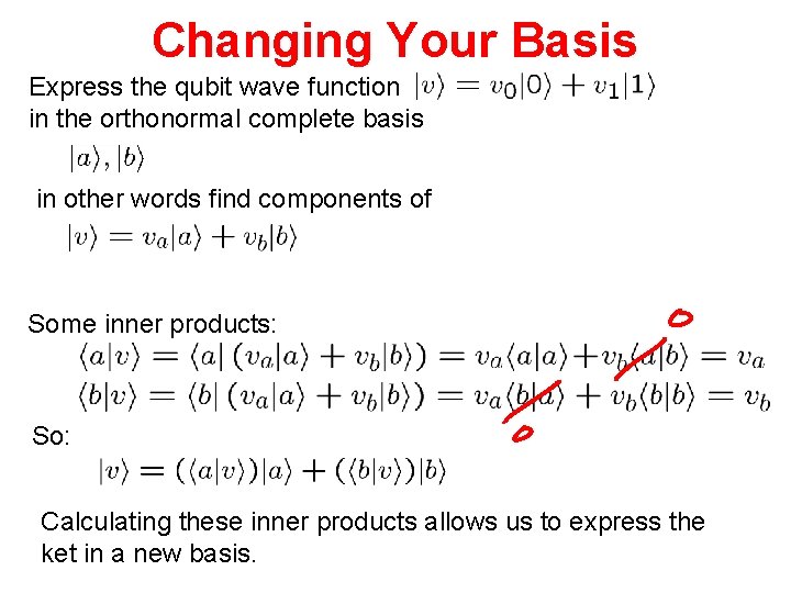
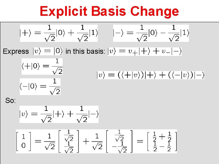
Changing Your Basis Express the qubit wave function in the orthonormal complete basis in other words find components of Some inner products: So: Calculating these inner products allows us to express the ket in a new basis.

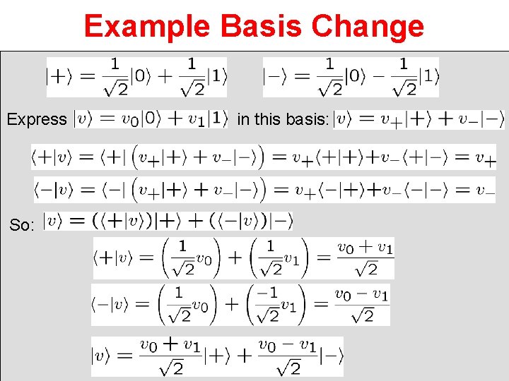
Example Basis Change Express So: in this basis:

Explicit Basis Change Express So: in this basis:

Linear Algebra Linear algebra is the language of quantum theory. We will need to develop some basic proficiency in order to work with quantum computers.

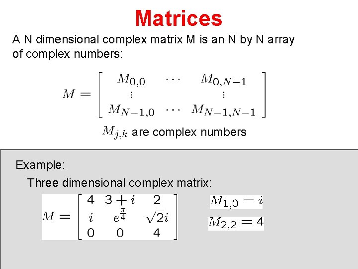
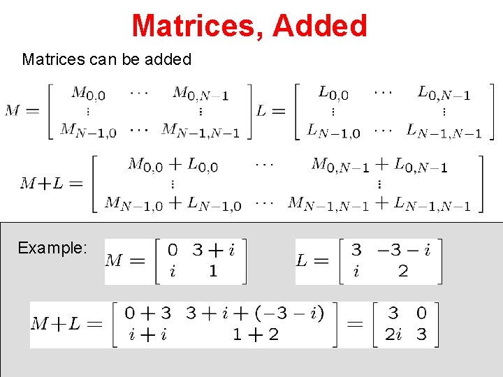
Matrices A N dimensional complex matrix M is an N by N array of complex numbers: are complex numbers Example: Three dimensional complex matrix:

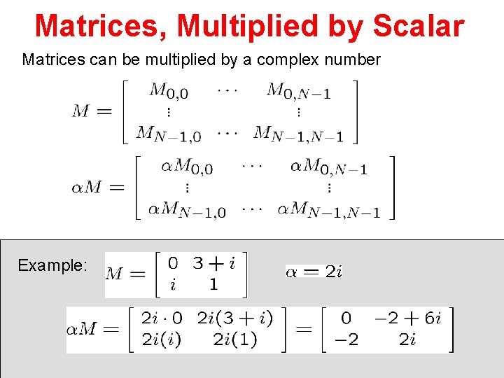
Matrices, Multiplied by Scalar Matrices can be multiplied by a complex number Example:

Matrices, Added Matrices can be added Example:

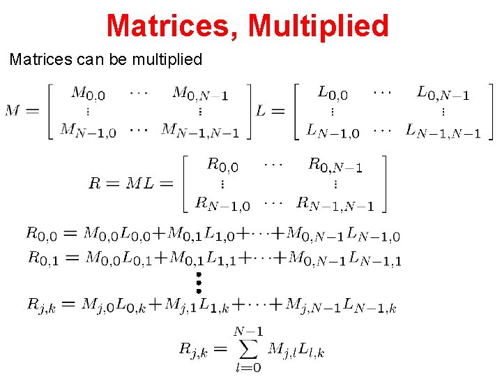
Matrices, Multiplied Matrices can be multiplied

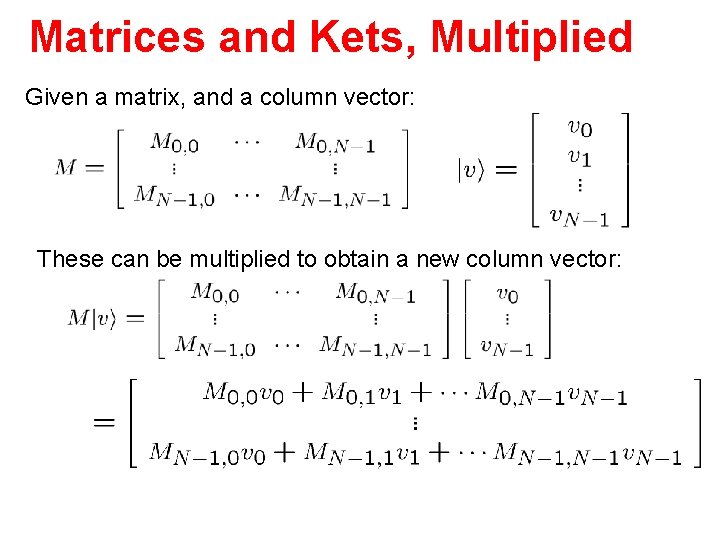
Matrices and Kets, Multiplied Given a matrix, and a column vector: These can be multiplied to obtain a new column vector:

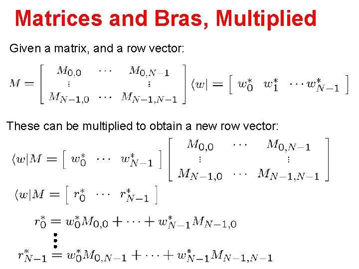
Matrices and Bras, Multiplied Given a matrix, and a row vector: These can be multiplied to obtain a new row vector:

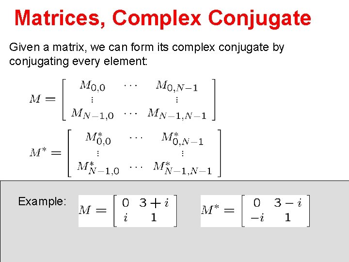
Matrices, Complex Conjugate Given a matrix, we can form its complex conjugate by conjugating every element: Example:

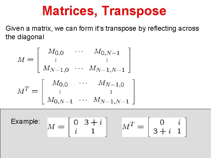
Matrices, Transpose Given a matrix, we can form it’s transpose by reflecting across the diagonal Example:

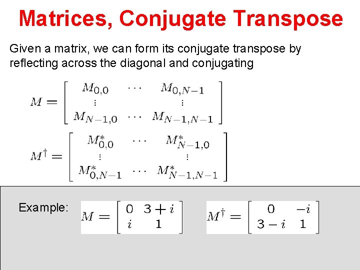
Matrices, Conjugate Transpose Given a matrix, we can form its conjugate transpose by reflecting across the diagonal and conjugating Example:

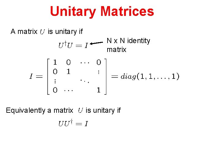
Unitary Matrices A matrix is unitary if N x N identity matrix Equivalently a matrix is unitary if

Quantum Rule 2: The wave function of a N dimensional quantum system evolves in time according to a unitary matrix. If the wave function initially is then after the evolution correspond to the new wave function is “Unitary Evolution”

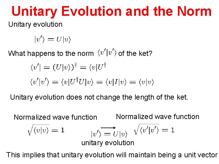
Unitary Evolution and the Norm Unitary evolution What happens to the norm of the ket? Unitary evolution does not change the length of the ket. Normalized wave function unitary evolution This implies that unitary evolution will maintain being a unit vector