Online Social Networks and Media Recommender Systems and


![Singular Value Decomposition • [n×m] = [n×r] [r×m] r: rank of matrix A Singular Value Decomposition • [n×m] = [n×r] [r×m] r: rank of matrix A](https://slidetodoc.com/presentation_image_h2/f1b2aabaa0fca5ce28259d6a555fa672/image-27.jpg)

- Slides: 79

Online Social Networks and Media Recommender Systems and Social Recommendations Thanks to: Jure Leskovec, Anand Rajaraman, Jeff Ullman

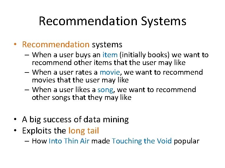
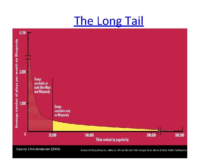
Recommendation Systems • Recommendation systems – When a user buys an item (initially books) we want to recommend other items that the user may like – When a user rates a movie, we want to recommend movies that the user may like – When a user likes a song, we want to recommend other songs that they may like • A big success of data mining • Exploits the long tail – How Into Thin Air made Touching the Void popular

The Long Tail Source: Chris Anderson (2004)

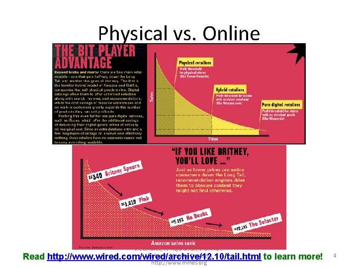
Physical vs. Online Read J. Leskovec, A. Rajaraman, J. Ullman: Mining of Massive Datasets, http: //www. wired. com/wired/archive/12. 10/tail. html http: //www. mmds. org to learn more! 4

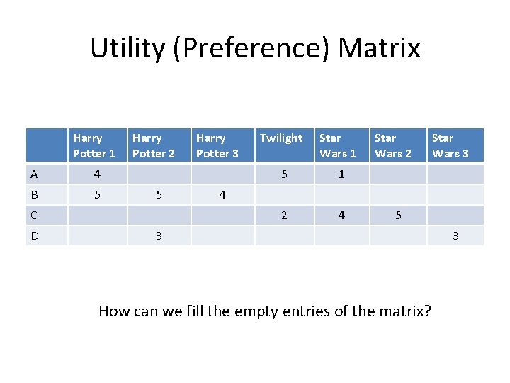
Utility (Preference) Matrix Harry Potter 1 A 4 B 5 Harry Potter 2 5 C D Harry Potter 3 Twilight Star Wars 1 5 1 2 4 Star Wars 2 Star Wars 3 4 5 3 How can we fill the empty entries of the matrix? 3

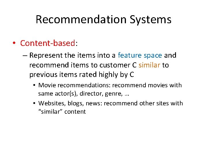
Recommendation Systems • Content-based: – Represent the items into a feature space and recommend items to customer C similar to previous items rated highly by C • Movie recommendations: recommend movies with same actor(s), director, genre, … • Websites, blogs, news: recommend other sites with “similar” content

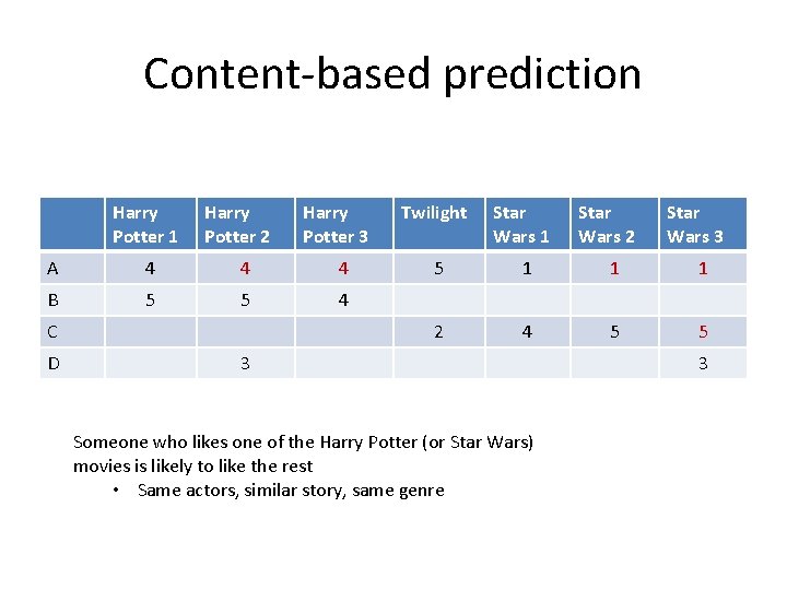
Content-based prediction Harry Potter 1 Harry Potter 2 Harry Potter 3 A 4 4 4 B 5 5 4 C D Twilight Star Wars 1 Star Wars 2 Star Wars 3 5 1 1 1 2 4 5 5 3 Someone who likes one of the Harry Potter (or Star Wars) movies is likely to like the rest • Same actors, similar story, same genre 3

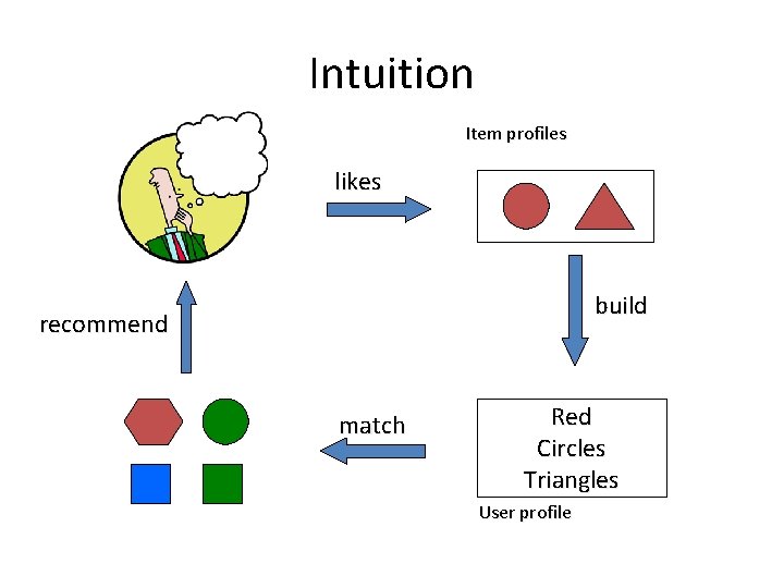
Intuition Item profiles likes build recommend match Red Circles Triangles User profile

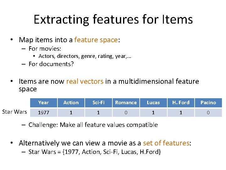
Extracting features for Items • Map items into a feature space: – For movies: • Actors, directors, genre, rating, year, … – For documents? • Items are now real vectors in a multidimensional feature space Star Wars Year Action Sci-Fi Romance Lucas H. Ford Pacino 1977 1 1 0 – Challenge: Make all feature values compatible • Alternatively we can view a movie as a set of features: – Star Wars = {1977, Action, Sci-Fi, Lucas, H. Ford}

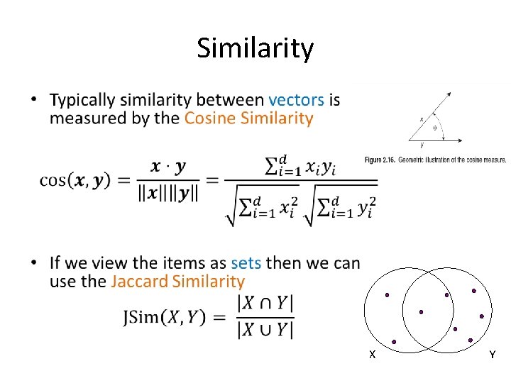
Extracting Features for Users • To compare items with users we need to map users to the same feature space. How? – Take all the movies that the user has seen and take the average vector • Other aggregation functions are also possible. • Recommend to user C the most similar item i computing similarity in the common feature space – How do we measure similarity?

Similarity • X Y

Classification approach • Using the user and item features we can construct a classifier that tries to predict if a user will like a new item

Limitations of content-based approach • Finding the appropriate features – e. g. , images, movies, music • Overspecialization – Never recommends items outside user’s content profile – People might have multiple interests

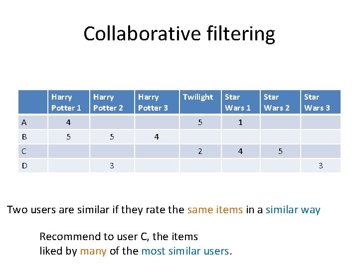
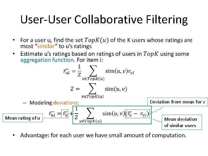
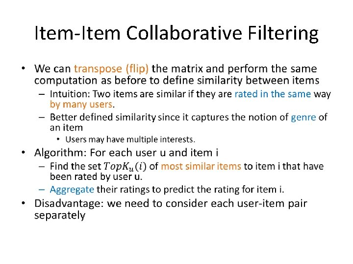
Collaborative filtering Harry Potter 1 A 4 B 5 Harry Potter 2 5 C D Harry Potter 3 Twilight Star Wars 1 5 1 2 4 Star Wars 2 Star Wars 3 4 3 5 3 Two users are similar if they rate the same items in a similar way Recommend to user C, the items liked by many of the most similar users.

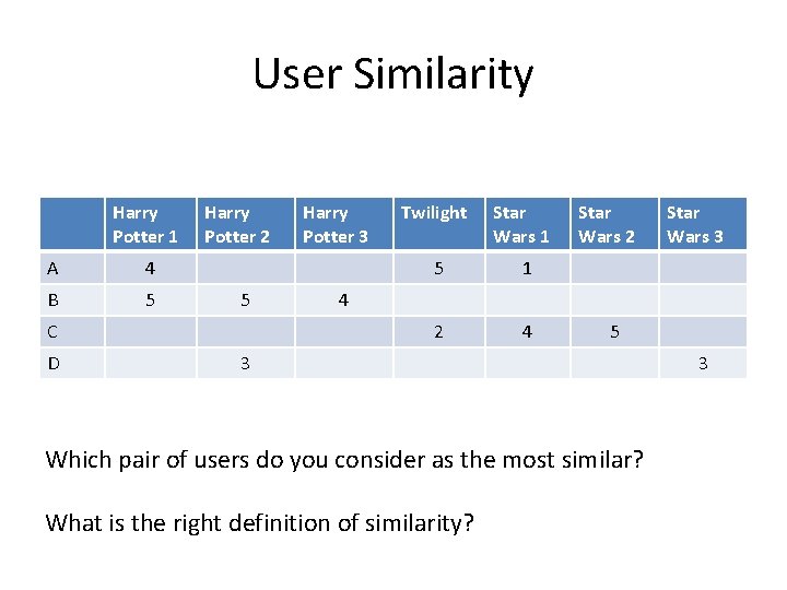
User Similarity Harry Potter 1 A 4 B 5 Harry Potter 2 5 C D Harry Potter 3 Twilight Star Wars 1 5 1 2 4 Star Wars 2 Star Wars 3 4 5 3 Which pair of users do you consider as the most similar? What is the right definition of similarity? 3

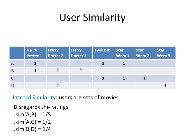
User Similarity Harry Potter 1 A 1 B 1 Harry Potter 2 1 C D Harry Potter 3 Twilight Star Wars 1 1 1 Star Wars 3 1 1 Jaccard Similarity: users are sets of movies Disregards the ratings. Jsim(A, B) = 1/5 Jsim(A, C) = 1/2 Jsim(B, D) = 1/4 Star Wars 2 1 1

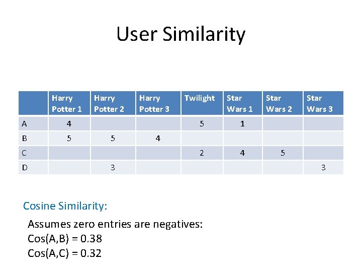
User Similarity Harry Potter 1 A 4 B 5 Harry Potter 2 5 C D Harry Potter 3 Twilight Star Wars 1 5 1 2 4 Star Wars 2 Star Wars 3 4 3 Cosine Similarity: Assumes zero entries are negatives: Cos(A, B) = 0. 38 Cos(A, C) = 0. 32 5 3

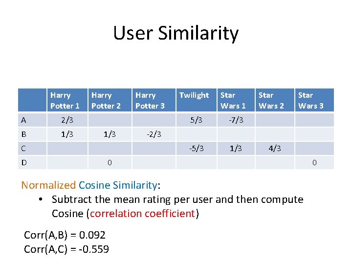
User Similarity Harry Potter 1 A 2/3 B 1/3 Harry Potter 2 1/3 C D Harry Potter 3 Twilight Star Wars 1 5/3 -7/3 -5/3 1/3 Star Wars 2 Star Wars 3 -2/3 4/3 0 Normalized Cosine Similarity: • Subtract the mean rating per user and then compute Cosine (correlation coefficient) Corr(A, B) = 0. 092 Corr(A, C) = -0. 559 0

User-User Collaborative Filtering • Deviation from mean for v Mean rating of u Mean deviation of similar users

Item-Item Collaborative Filtering •

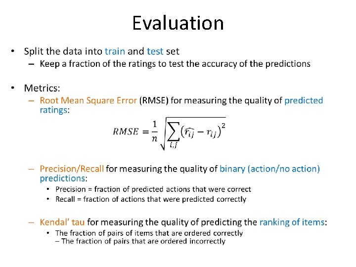
Evaluation •

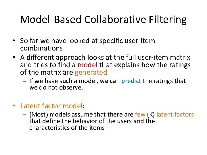
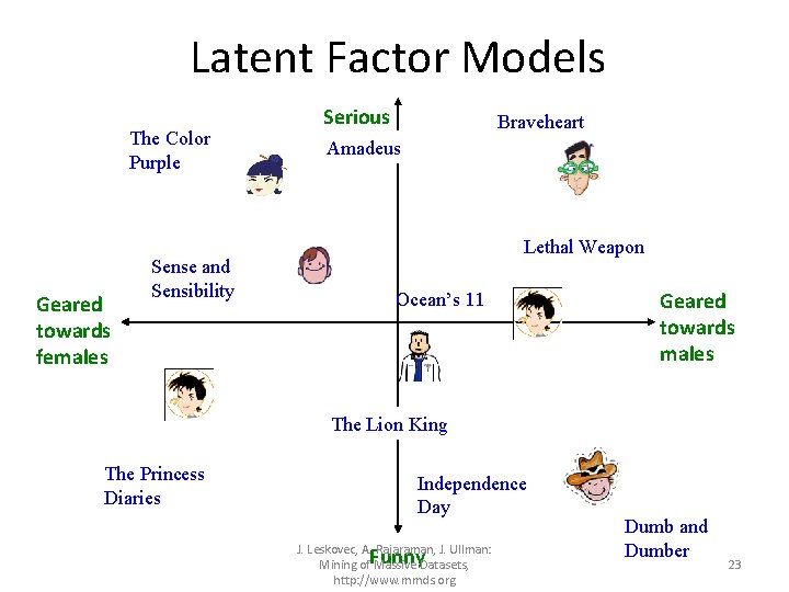
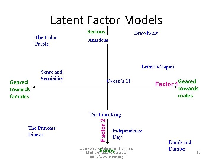
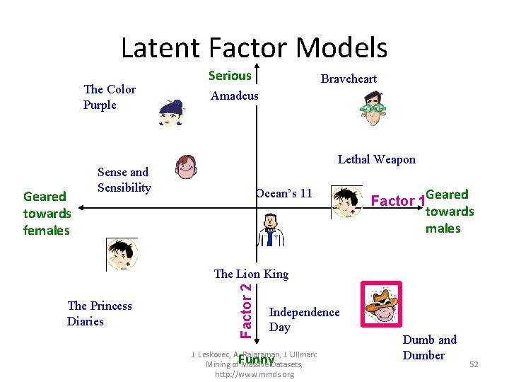
Model-Based Collaborative Filtering • So far we have looked at specific user-item combinations • A different approach looks at the full user-item matrix and tries to find a model that explains how the ratings of the matrix are generated – If we have such a model, we can predict the ratings that we do not observe. • Latent factor model: – (Most) models assume that there are few (K) latent factors that define the behavior of the users and the characteristics of the items

Latent Factor Models The Color Purple Geared towards females Sense and Sensibility Serious Braveheart Amadeus Lethal Weapon Ocean’s 11 Geared towards males The Lion King The Princess Diaries Independence Day J. Leskovec, A. Rajaraman, J. Ullman: Mining of Massive Datasets, http: //www. mmds. org Funny Dumb and Dumber 23

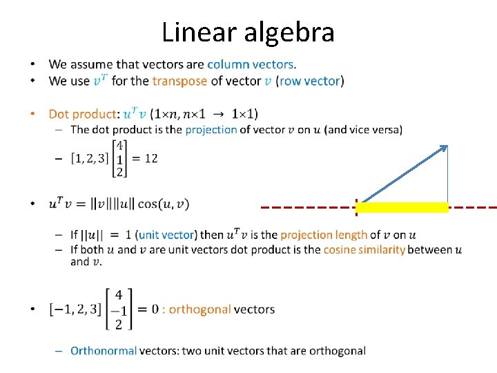
Linear algebra •

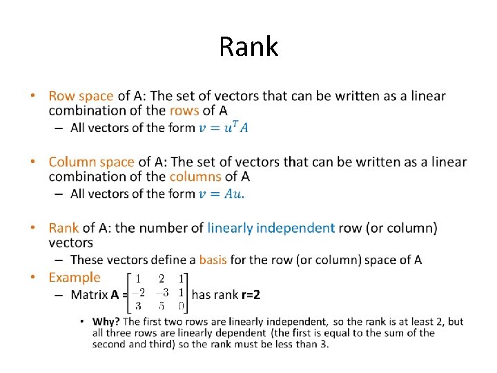
Rank •

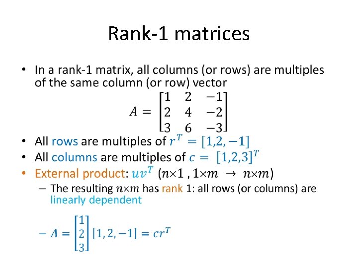
Rank-1 matrices •
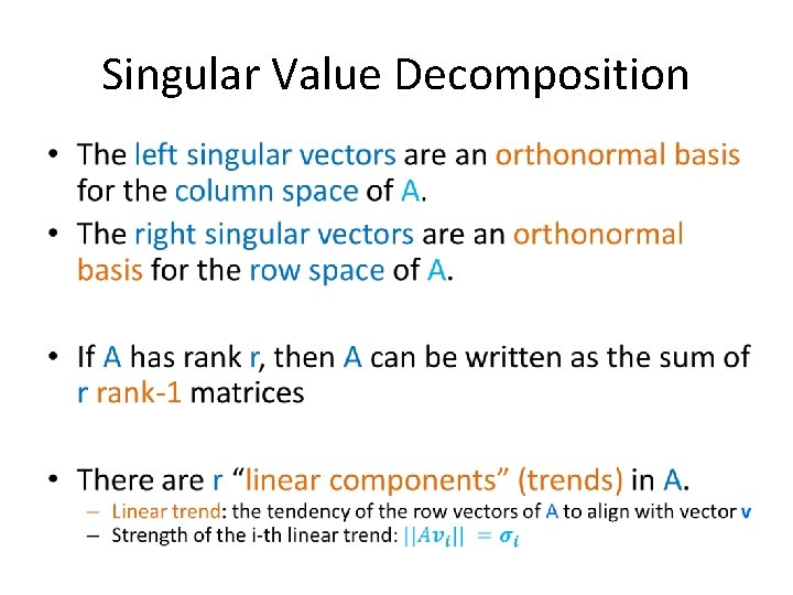
![Singular Value Decomposition nm nr rm r rank of matrix A Singular Value Decomposition • [n×m] = [n×r] [r×m] r: rank of matrix A](https://slidetodoc.com/presentation_image_h2/f1b2aabaa0fca5ce28259d6a555fa672/image-27.jpg)
Singular Value Decomposition • [n×m] = [n×r] [r×m] r: rank of matrix A

Singular Value Decomposition •

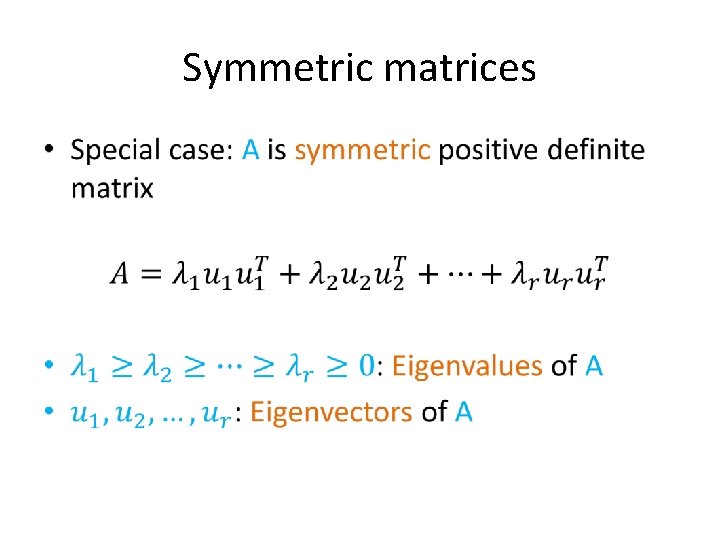
Symmetric matrices •

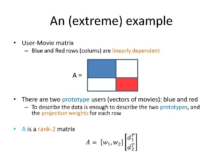
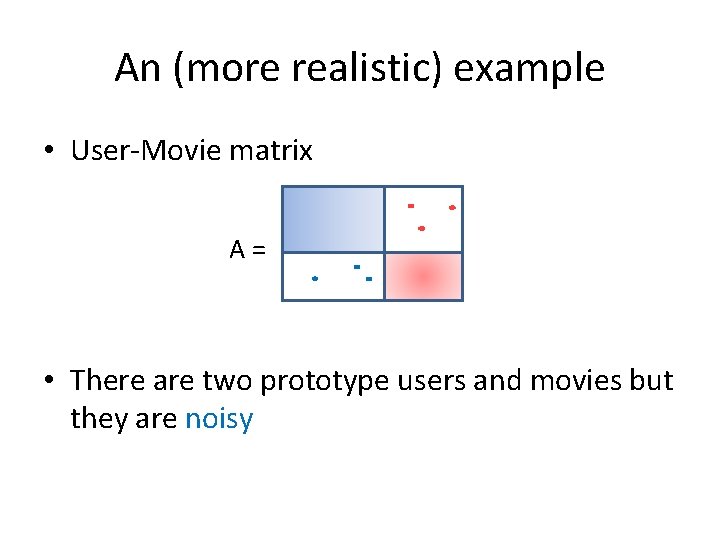
An (extreme) example • A=

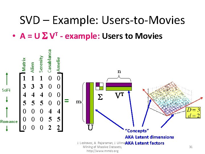
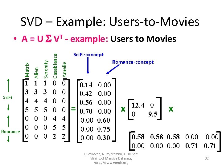
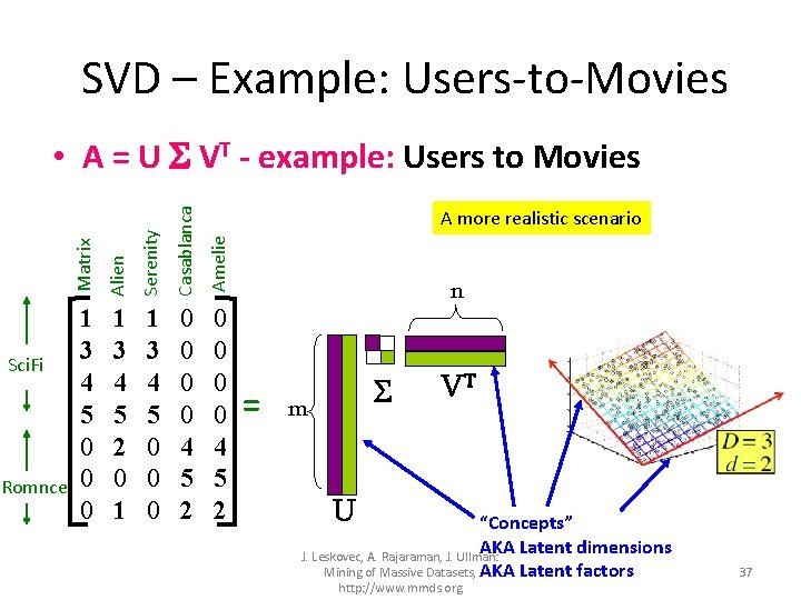
SVD – Example: Users-to-Movies Serenity Casablanca Amelie Romance Alien Sci. Fi Matrix • A = U VT - example: Users to Movies 1 3 4 5 0 0 0 0 4 5 2 0 0 4 5 2 n = m VT U “Concepts” AKA Latent dimensions J. Leskovec, A. Rajaraman, J. Ullman: AKA Latent factors Mining of Massive Datasets, http: //www. mmds. org 31

SVD – Example: Users-to-Movies • A = U VT - example: Users to Movies Alien Serenity Casablanca Amelie Romance Matrix Sci. Fi-concept 1 3 4 5 0 0 0 0 4 5 2 0 0 4 5 2 Romance-concept = 0. 14 0. 42 0. 56 0. 70 0. 00 0. 60 0. 75 0. 30 x 12. 4 0 0 9. 5 x 0. 58 0. 00 0. 71 J. Leskovec, A. Rajaraman, J. Ullman: Mining of Massive Datasets, http: //www. mmds. org 32

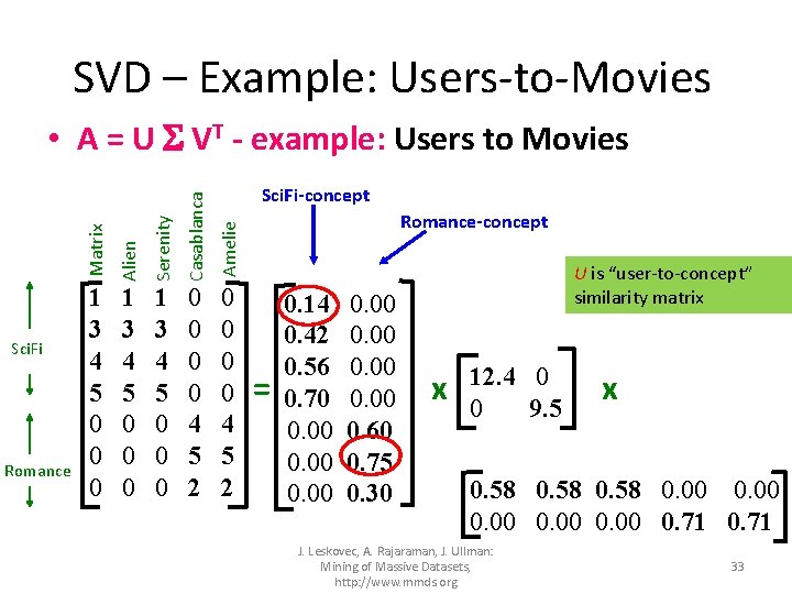
SVD – Example: Users-to-Movies • A = U VT - example: Users to Movies Alien Serenity Casablanca Amelie Romance Matrix Sci. Fi-concept 1 3 4 5 0 0 0 0 4 5 2 0 0 4 5 2 Romance-concept = 0. 14 0. 42 0. 56 0. 70 0. 00 0. 60 0. 75 0. 30 U is “user-to-concept” similarity matrix x 12. 4 0 0 9. 5 x 0. 58 0. 00 0. 71 J. Leskovec, A. Rajaraman, J. Ullman: Mining of Massive Datasets, http: //www. mmds. org 33

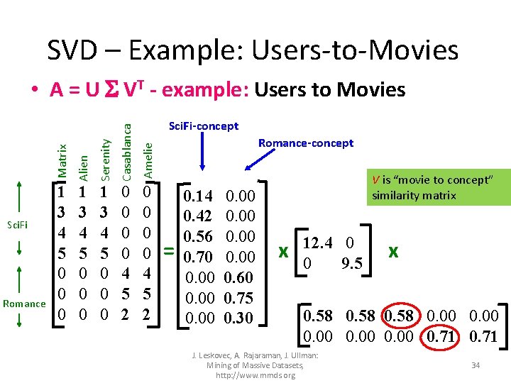
SVD – Example: Users-to-Movies • A = U VT - example: Users to Movies Alien Serenity Casablanca Amelie Romance Matrix Sci. Fi-concept 1 3 4 5 0 0 0 0 4 5 2 0 0 4 5 2 Romance-concept = 0. 14 0. 42 0. 56 0. 70 0. 00 0. 60 0. 75 0. 30 V is “movie to concept” similarity matrix x 12. 4 0 0 9. 5 x 0. 58 0. 00 0. 71 J. Leskovec, A. Rajaraman, J. Ullman: Mining of Massive Datasets, http: //www. mmds. org 34

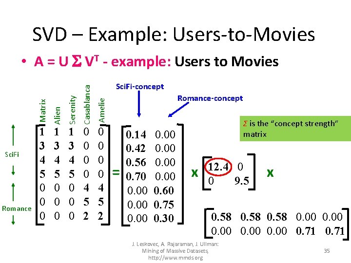
SVD – Example: Users-to-Movies • A = U VT - example: Users to Movies Alien Serenity Casablanca Amelie Romance Matrix Sci. Fi-concept 1 3 4 5 0 0 0 0 4 5 2 0 0 4 5 2 Romance-concept = 0. 14 0. 42 0. 56 0. 70 0. 00 0. 60 0. 75 0. 30 Σ is the “concept strength” matrix x 12. 4 0 0 9. 5 x 0. 58 0. 00 0. 71 J. Leskovec, A. Rajaraman, J. Ullman: Mining of Massive Datasets, http: //www. mmds. org 35

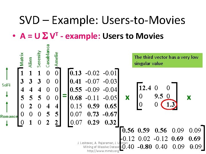
An (more realistic) example • User-Movie matrix A= • There are two prototype users and movies but they are noisy

SVD – Example: Users-to-Movies Serenity Casablanca Amelie Romnce Alien Sci. Fi Matrix • A = U VT - example: Users to Movies 1 3 4 5 0 0 0 1 3 4 5 2 0 1 1 3 4 5 0 0 0 0 4 5 2 A more realistic scenario n = m VT U “Concepts” AKA Latent dimensions J. Leskovec, A. Rajaraman, J. Ullman: Mining of Massive Datasets, AKA Latent factors http: //www. mmds. org 37

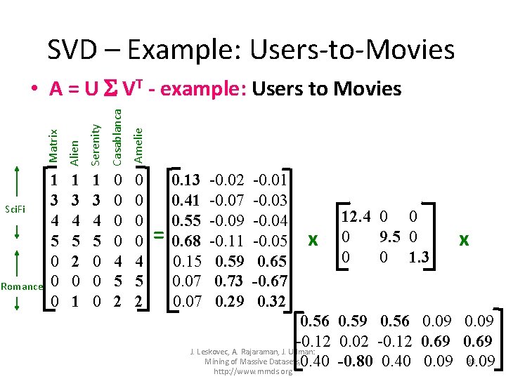
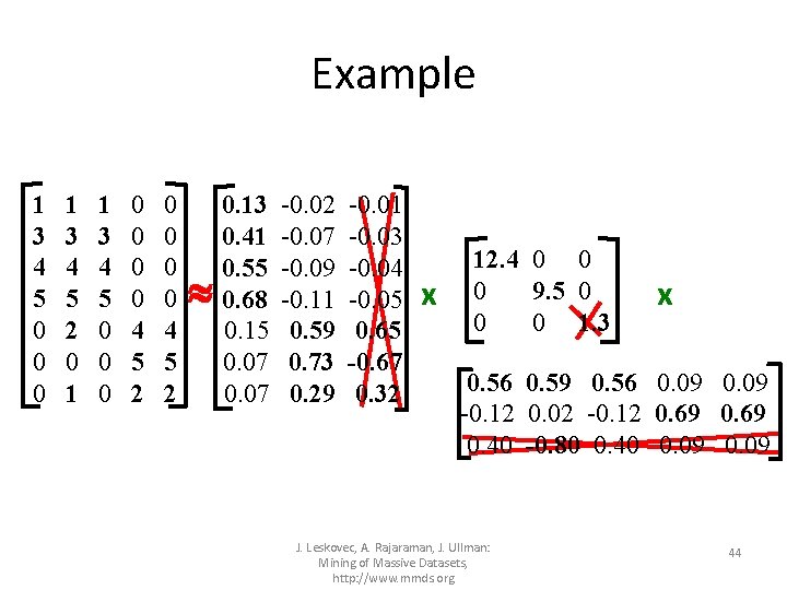
SVD – Example: Users-to-Movies Serenity Casablanca Amelie Romance Alien Sci. Fi Matrix • A = U VT - example: Users to Movies 1 3 4 5 0 0 0 1 3 4 5 2 0 1 1 3 4 5 0 0 0 0 4 5 2 = 0. 13 0. 41 0. 55 0. 68 0. 15 0. 07 -0. 02 -0. 07 -0. 09 -0. 11 0. 59 0. 73 0. 29 -0. 01 -0. 03 -0. 04 -0. 05 0. 65 -0. 67 0. 32 x 12. 4 0 0 0 9. 5 0 0 0 1. 3 x 0. 56 0. 59 0. 56 0. 09 -0. 12 0. 02 -0. 12 0. 69 J. Leskovec, A. Rajaraman, J. Ullman: 38 Mining of Massive Datasets, 0. 40 -0. 80 0. 40 0. 09 http: //www. mmds. org

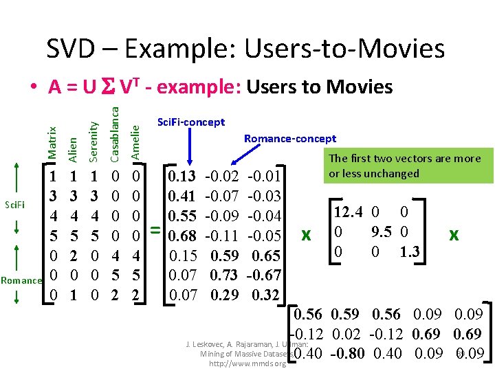
SVD – Example: Users-to-Movies Serenity Casablanca Amelie Romance Alien Sci. Fi Matrix • A = U VT - example: Users to Movies 1 3 4 5 0 0 0 1 3 4 5 2 0 1 1 3 4 5 0 0 0 0 4 5 2 Sci. Fi-concept Romance-concept = 0. 13 0. 41 0. 55 0. 68 0. 15 0. 07 -0. 02 -0. 07 -0. 09 -0. 11 0. 59 0. 73 0. 29 -0. 01 -0. 03 -0. 04 -0. 05 0. 65 -0. 67 0. 32 The first two vectors are more or less unchanged x 12. 4 0 0 0 9. 5 0 0 0 1. 3 x 0. 56 0. 59 0. 56 0. 09 -0. 12 0. 02 -0. 12 0. 69 J. Leskovec, A. Rajaraman, J. Ullman: 39 Mining of Massive Datasets, 0. 40 -0. 80 0. 40 0. 09 http: //www. mmds. org

SVD – Example: Users-to-Movies Serenity Casablanca Amelie Romance Alien Sci. Fi Matrix • A = U VT - example: Users to Movies 1 3 4 5 0 0 0 1 3 4 5 2 0 1 1 3 4 5 0 0 0 0 4 5 2 The third vector has a very low singular value = 0. 13 0. 41 0. 55 0. 68 0. 15 0. 07 -0. 02 -0. 07 -0. 09 -0. 11 0. 59 0. 73 0. 29 -0. 01 -0. 03 -0. 04 -0. 05 0. 65 -0. 67 0. 32 x 12. 4 0 0 0 9. 5 0 0 0 1. 3 x 0. 56 0. 59 0. 56 0. 09 -0. 12 0. 02 -0. 12 0. 69 J. Leskovec, A. Rajaraman, J. Ullman: 40 Mining of Massive Datasets, 0. 40 -0. 80 0. 40 0. 09 http: //www. mmds. org

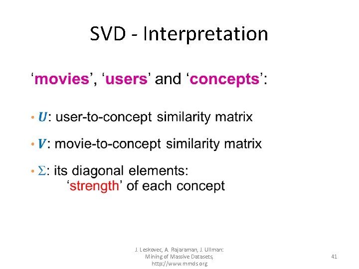
SVD - Interpretation • J. Leskovec, A. Rajaraman, J. Ullman: Mining of Massive Datasets, http: //www. mmds. org 41

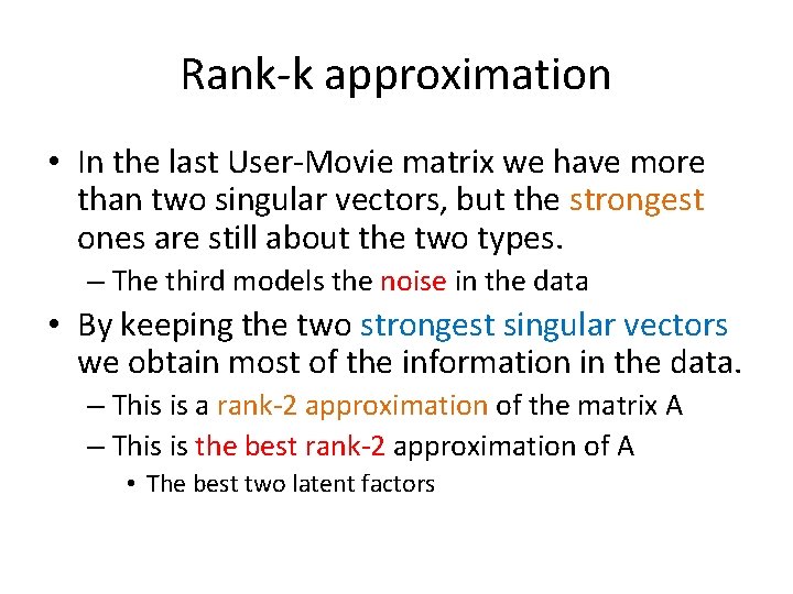
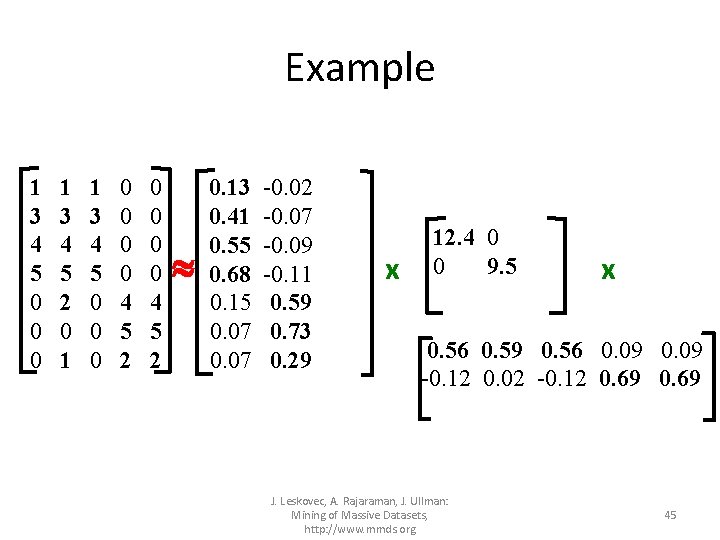
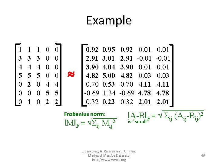
Rank-k approximation • In the last User-Movie matrix we have more than two singular vectors, but the strongest ones are still about the two types. – The third models the noise in the data • By keeping the two strongest singular vectors we obtain most of the information in the data. – This is a rank-2 approximation of the matrix A – This is the best rank-2 approximation of A • The best two latent factors

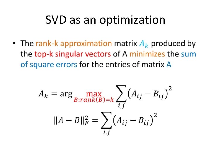
SVD as an optimization •

Example 1 3 4 5 0 0 0 1 3 4 5 2 0 1 1 3 4 5 0 0 0 0 4 5 2 0. 13 0. 41 0. 55 0. 68 0. 15 0. 07 -0. 02 -0. 07 -0. 09 -0. 11 0. 59 0. 73 0. 29 -0. 01 -0. 03 -0. 04 -0. 05 0. 65 -0. 67 0. 32 x 12. 4 0 0 0 9. 5 0 0 0 1. 3 x 0. 56 0. 59 0. 56 0. 09 -0. 12 0. 02 -0. 12 0. 69 0. 40 -0. 80 0. 40 0. 09 J. Leskovec, A. Rajaraman, J. Ullman: Mining of Massive Datasets, http: //www. mmds. org 44

Example 1 3 4 5 0 0 0 1 3 4 5 2 0 1 1 3 4 5 0 0 0 0 4 5 2 0. 13 0. 41 0. 55 0. 68 0. 15 0. 07 -0. 02 -0. 07 -0. 09 -0. 11 0. 59 0. 73 0. 29 x 12. 4 0 0 9. 5 x 0. 56 0. 59 0. 56 0. 09 -0. 12 0. 02 -0. 12 0. 69 J. Leskovec, A. Rajaraman, J. Ullman: Mining of Massive Datasets, http: //www. mmds. org 45

Example 1 3 4 5 0 0 0 1 3 4 5 2 0 1 1 3 4 5 0 0 0 0 4 5 2 0. 92 2. 91 3. 90 4. 82 0. 70 -0. 69 0. 32 0. 95 3. 01 4. 04 5. 00 0. 53 1. 34 0. 23 Frobenius norm: ǁMǁF = Σij Mij 2 0. 92 2. 91 3. 90 4. 82 0. 70 -0. 69 0. 32 0. 01 -0. 01 0. 03 4. 11 4. 78 2. 01 ǁA-BǁF = Σij (Aij-Bij)2 is “small” J. Leskovec, A. Rajaraman, J. Ullman: Mining of Massive Datasets, http: //www. mmds. org 46

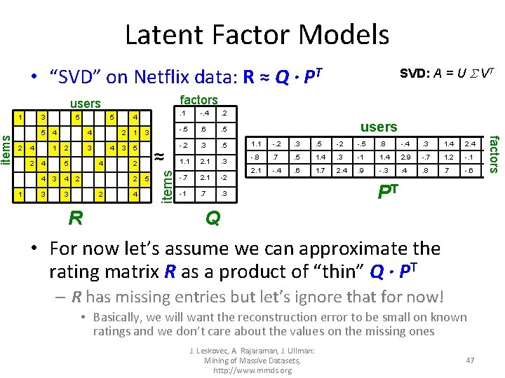
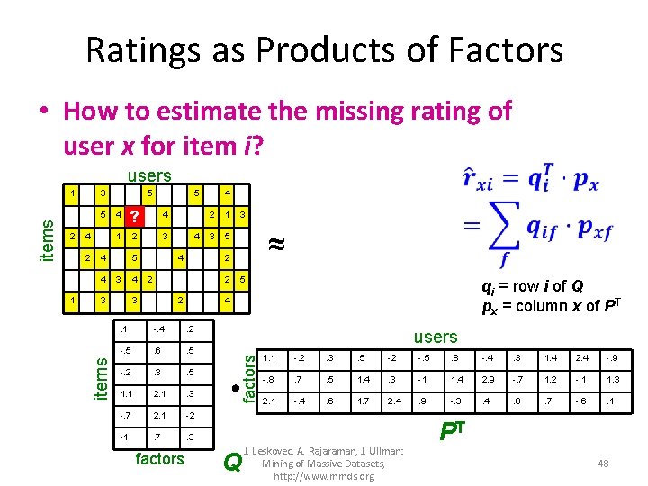
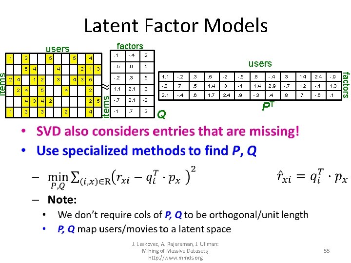
• “SVD” on Netflix data: R ≈ Q · PT factors users 3 5 2 4 3 5 4 1 5 4 2 3 5 3 4 4 4 2 1 3 5 2 R ≈ 2 2 3 3 4 5 items 1 SVD: A = U VT . 1 -. 4 . 2 -. 5 . 6 . 5 -. 2 . 3 . 5 1. 1 2. 1 . 3 -. 7 2. 1 -2 -1 . 7 . 3 users factors items Latent Factor Models 1. 1 -. 2 . 3 . 5 -2 -. 5 . 8 -. 4 . 3 1. 4 2. 4 -. 9 -. 8 . 7 . 5 1. 4 . 3 -1 1. 4 2. 9 -. 7 1. 2 -. 1 1. 3 2. 1 -. 4 . 6 1. 7 2. 4 . 9 -. 3 . 4 . 8 . 7 -. 6 . 1 PT Q • For now let’s assume we can approximate the rating matrix R as a product of “thin” Q · PT – R has missing entries but let’s ignore that for now! • Basically, we will want the reconstruction error to be small on known ratings and we don’t care about the values on the missing ones J. Leskovec, A. Rajaraman, J. Ullman: Mining of Massive Datasets, http: //www. mmds. org 47

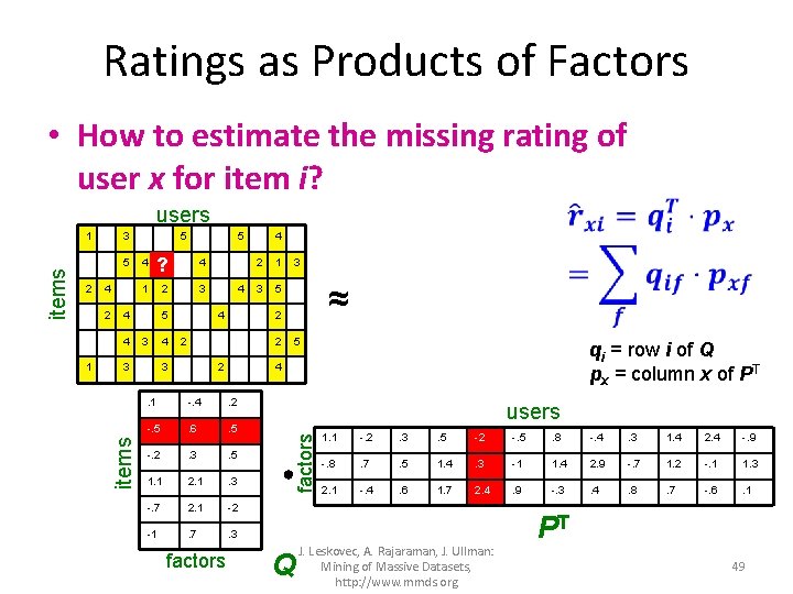
Ratings as Products of Factors • How to estimate the missing rating of user x for item i? users 5 2 4 2 5 4 ? 4 1 2 3 4 4 1 5 5 3 3 4 4 2 1 3 5 2 2 5 qi = row i of Q px = column x of PT 4 . 1 -. 4 . 2 -. 5 . 6 . 5 -. 2 . 3 . 5 1. 1 2. 1 . 3 -. 7 2. 1 -2 -1 . 7 . 3 factors ≈ 2 2 3 3 users factors 3 items 1 Q 1. 1 -. 2 . 3 . 5 -2 -. 5 . 8 -. 4 . 3 1. 4 2. 4 -. 9 -. 8 . 7 . 5 1. 4 . 3 -1 1. 4 2. 9 -. 7 1. 2 -. 1 1. 3 2. 1 -. 4 . 6 1. 7 2. 4 . 9 -. 3 . 4 . 8 . 7 -. 6 . 1 J. Leskovec, A. Rajaraman, J. Ullman: Mining of Massive Datasets, http: //www. mmds. org PT 48

Ratings as Products of Factors • How to estimate the missing rating of user x for item i? users 5 2 4 2 5 4 ? 4 1 2 3 4 4 1 5 5 3 3 4 4 2 1 3 5 2 2 5 qi = row i of Q px = column x of PT 4 . 1 -. 4 . 2 -. 5 . 6 . 5 -. 2 . 3 . 5 1. 1 2. 1 . 3 -. 7 2. 1 -2 -1 . 7 . 3 factors ≈ 2 2 3 3 users factors 3 items 1 Q 1. 1 -. 2 . 3 . 5 -2 -. 5 . 8 -. 4 . 3 1. 4 2. 4 -. 9 -. 8 . 7 . 5 1. 4 . 3 -1 1. 4 2. 9 -. 7 1. 2 -. 1 1. 3 2. 1 -. 4 . 6 1. 7 2. 4 . 9 -. 3 . 4 . 8 . 7 -. 6 . 1 J. Leskovec, A. Rajaraman, J. Ullman: Mining of Massive Datasets, http: //www. mmds. org PT 49

Ratings as Products of Factors • How to estimate the missing rating of user x for item i? users 5 2 4 2 5 4 2. 4 ? 4 1 2 3 4 4 1 5 5 3 3 4 4 2 1 3 5 ≈ 2 2 2 3 3 2 5 qi = row i of Q px = column x of PT 4 . 1 -. 4 . 2 -. 5 . 6 . 5 -. 2 . 3 . 5 1. 1 2. 1 . 3 -. 7 2. 1 -2 -1 . 7 . 3 f factors users f factors 3 items 1 Q 1. 1 -. 2 . 3 . 5 -2 -. 5 . 8 -. 4 . 3 1. 4 2. 4 -. 9 -. 8 . 7 . 5 1. 4 . 3 -1 1. 4 2. 9 -. 7 1. 2 -. 1 1. 3 2. 1 -. 4 . 6 1. 7 2. 4 . 9 -. 3 . 4 . 8 . 7 -. 6 . 1 J. Leskovec, A. Rajaraman, J. Ullman: Mining of Massive Datasets, http: //www. mmds. org PT 50

Latent Factor Models The Color Purple Geared towards females Serious Braveheart Amadeus Lethal Weapon Sense and Sensibility Ocean’s 11 Geared Factor 1 towards males The Princess Diaries Factor 2 The Lion King Independence Day J. Leskovec, A. Rajaraman, J. Ullman: Mining of Massive Datasets, http: //www. mmds. org Funny Dumb and Dumber 51

Latent Factor Models The Color Purple Geared towards females Serious Braveheart Amadeus Lethal Weapon Sense and Sensibility Ocean’s 11 Geared Factor 1 towards males The Princess Diaries Factor 2 The Lion King Independence Day J. Leskovec, A. Rajaraman, J. Ullman: Mining of Massive Datasets, http: //www. mmds. org Funny Dumb and Dumber 52

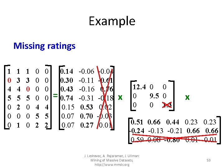
Example Missing ratings 1 0 4 5 0 0 0 1 3 4 5 2 0 1 1 3 0 5 0 0 0 0 4 5 2 0. 14 0. 30 0. 43 = 0. 74 0. 15 0. 07 -0. 06 -0. 04 -0. 11 -0. 61 -0. 16 0. 76 -0. 31 -0. 18 0. 53 0. 02 0. 70 -0. 03 0. 27 0. 01 x 12. 4 0 0 0 9. 5 0 0 0 1. 3 x 0. 51 0. 66 0. 44 0. 23 -0. 24 -0. 13 -0. 21 0. 66 0. 59 0. 08 -0. 80 0. 01 J. Leskovec, A. Rajaraman, J. Ullman: Mining of Massive Datasets, http: //www. mmds. org 53

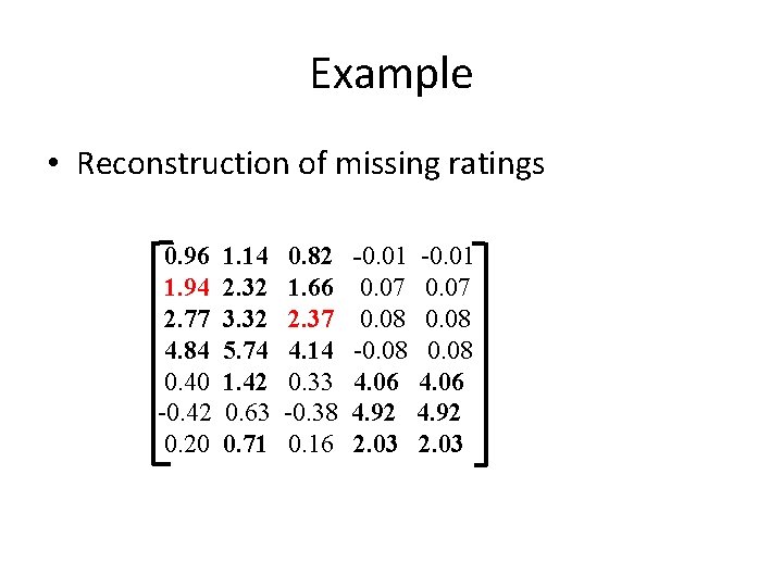
Example • Reconstruction of missing ratings 0. 96 1. 94 2. 77 4. 84 0. 40 -0. 42 0. 20 1. 14 2. 32 3. 32 5. 74 1. 42 0. 63 0. 71 0. 82 1. 66 2. 37 4. 14 0. 33 -0. 38 0. 16 -0. 01 0. 07 0. 08 -0. 08 4. 06 4. 92 2. 03 -0. 01 0. 07 0. 08 4. 06 4. 92 2. 03

factors 1 3 5 2 4 1 4 4 1 5 3 4 2 3 5 4 3 4 4 2 -. 4 . 2 -. 5 . 6 . 5 -. 2 . 3 . 5 1. 1 2. 1 . 3 -. 7 2. 1 -2 -1 . 7 . 3 4 2 1 3 5 3 2 2 2 . 1 items users 4 5 users 1. 1 -. 2 . 3 . 5 -2 -. 5 . 8 -. 4 . 3 1. 4 2. 4 -. 9 -. 8 . 7 . 5 1. 4 . 3 -1 1. 4 2. 9 -. 7 1. 2 -. 1 1. 3 2. 1 -. 4 . 6 1. 7 2. 4 . 9 -. 3 . 4 . 8 . 7 -. 6 . 1 Q PT • J. Leskovec, A. Rajaraman, J. Ullman: Mining of Massive Datasets, http: //www. mmds. org 55 factors items Latent Factor Models

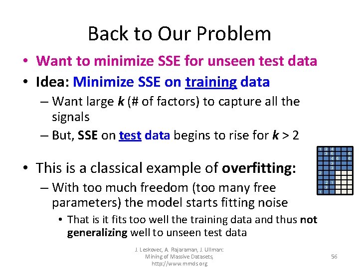
Back to Our Problem • Want to minimize SSE for unseen test data • Idea: Minimize SSE on training data – Want large k (# of factors) to capture all the signals – But, SSE on test data begins to rise for k > 2 • This is a classical example of overfitting: – With too much freedom (too many free parameters) the model starts fitting noise 1 3 4 3 5 4 5 3 3 2 ? ? ? 2 1 3 1 • That is it fits too well the training data and thus not generalizing well to unseen test data J. Leskovec, A. Rajaraman, J. Ullman: Mining of Massive Datasets, http: //www. mmds. org 5 5 56 ? ?

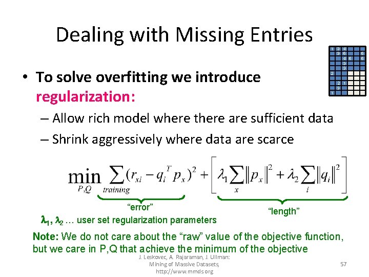
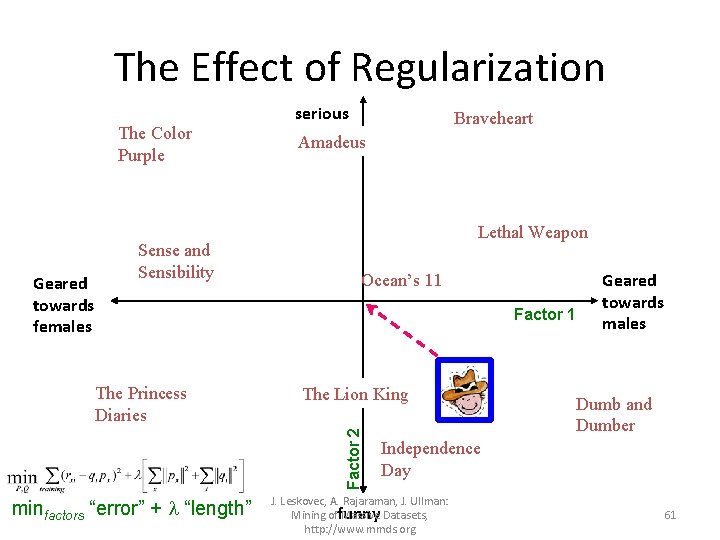
Dealing with Missing Entries • To solve overfitting we introduce regularization: 1 3 4 3 5 4 5 3 3 2 ? 2 1 3 1 “length” Note: We do not care about the “raw” value of the objective function, but we care in P, Q that achieve the minimum of the objective J. Leskovec, A. Rajaraman, J. Ullman: Mining of Massive Datasets, http: //www. mmds. org ? ? – Allow rich model where there are sufficient data – Shrink aggressively where data are scarce “error” 1, 2 … user set regularization parameters 5 5 57 ? ?

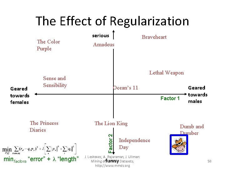
The Effect of Regularization The Color Purple Geared towards females Sense and Sensibility serious Braveheart Amadeus Lethal Weapon Ocean’s 11 Factor 1 The Lion King Factor 2 The Princess Diaries minfactors “error” + “length” Geared towards males Dumb and Dumber Independence Day J. Leskovec, A. Rajaraman, J. Ullman: Mining offunny Massive Datasets, http: //www. mmds. org 58

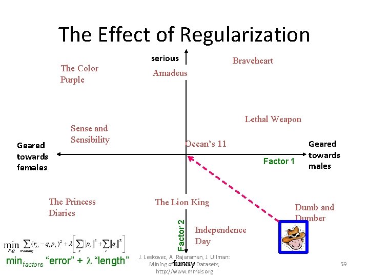
The Effect of Regularization The Color Purple Geared towards females Sense and Sensibility serious Braveheart Amadeus Lethal Weapon Ocean’s 11 Factor 1 The Lion King Factor 2 The Princess Diaries minfactors “error” + “length” Geared towards males Dumb and Dumber Independence Day J. Leskovec, A. Rajaraman, J. Ullman: Mining offunny Massive Datasets, http: //www. mmds. org 59

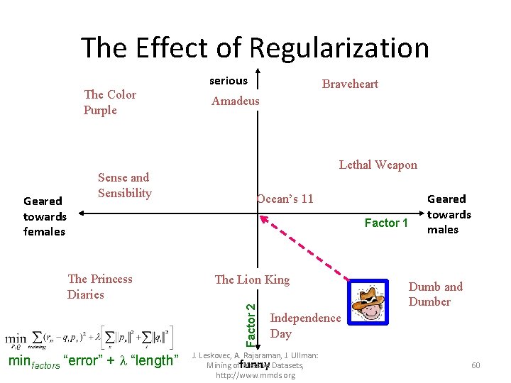
The Effect of Regularization The Color Purple Geared towards females Sense and Sensibility serious Braveheart Amadeus Lethal Weapon Ocean’s 11 Factor 1 The Lion King Factor 2 The Princess Diaries minfactors “error” + “length” Geared towards males Dumb and Dumber Independence Day J. Leskovec, A. Rajaraman, J. Ullman: Mining offunny Massive Datasets, http: //www. mmds. org 60

The Effect of Regularization The Color Purple Geared towards females Sense and Sensibility serious Braveheart Amadeus Lethal Weapon Ocean’s 11 Factor 1 The Lion King Factor 2 The Princess Diaries minfactors “error” + “length” Geared towards males Dumb and Dumber Independence Day J. Leskovec, A. Rajaraman, J. Ullman: Mining offunny Massive Datasets, http: //www. mmds. org 61

Latent factors • To find the P, Q that minimize the error function we can use (stochastic) gradient descent • We can define different latent factor models that apply the same idea in different ways – Probabilistic/Generative models. • The latent factor methods work well in practice, and they are employed by most sophisticated recommendation systems

Pros and cons of collaborative filtering • Works for any kind of item – No feature selection needed • Cold-Start problem: – New user problem – New item problem • Sparsity of rating matrix – Cluster-based smoothing?

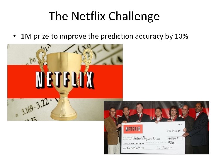
The Netflix Challenge • 1 M prize to improve the prediction accuracy by 10%

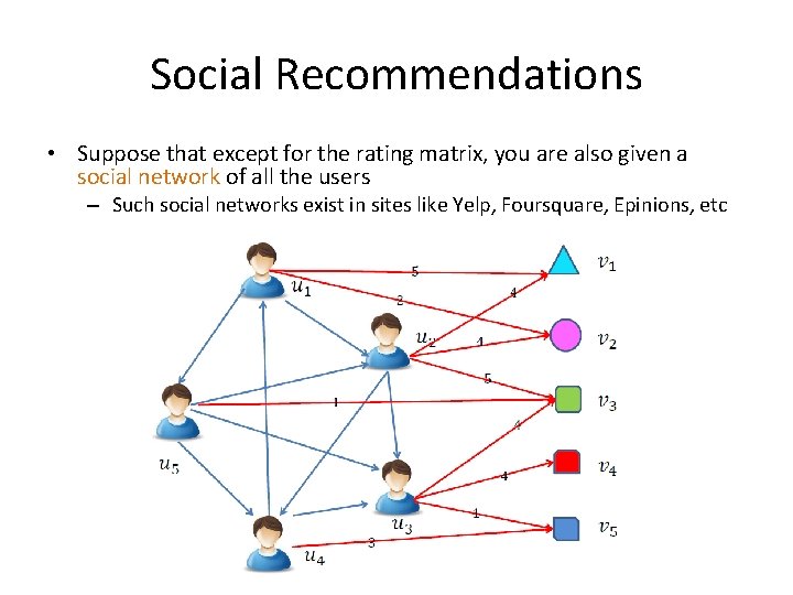
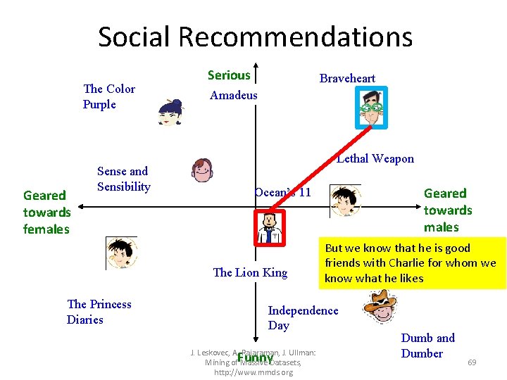
Social Recommendations • Suppose that except for the rating matrix, you are also given a social network of all the users – Such social networks exist in sites like Yelp, Foursquare, Epinions, etc

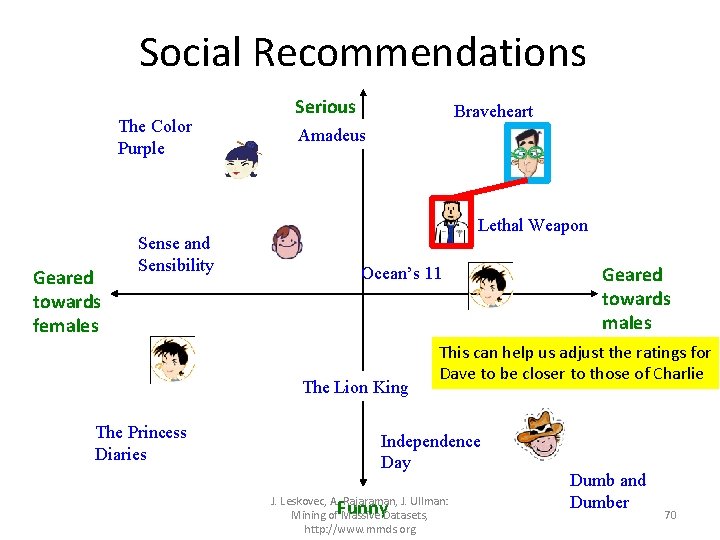
Social Recommendations • How can we use the social network to improve recommendations? – Homophily: connected users are likely to have similar ratings.

Social Recommendations • Ideas? – For a user who has no ratings, but has friends take the average of the friends to be the predicted rating • Use relationship strength when available – Combine the rating similarity and neighborhood rating to predict rating. – Use social network to determine similarity between users.

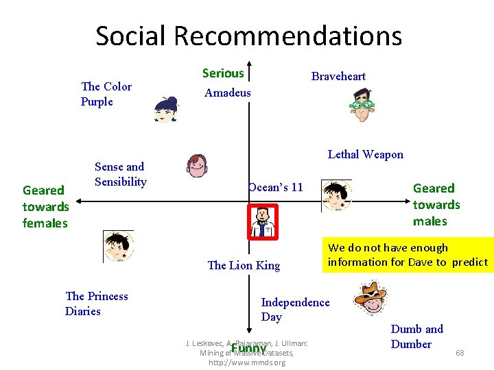
Social Recommendations The Color Purple Geared towards females Sense and Sensibility Serious Braveheart Amadeus Lethal Weapon The Lion King The Princess Diaries Geared towards males Ocean’s 11 We do not have enough information for Dave to predict Independence Day J. Leskovec, A. Rajaraman, J. Ullman: Mining of Massive Datasets, http: //www. mmds. org Funny Dumb and Dumber 68

Social Recommendations The Color Purple Geared towards females Sense and Sensibility Serious Braveheart Amadeus Lethal Weapon The Lion King The Princess Diaries Geared towards males Ocean’s 11 But we know that he is good friends with Charlie for whom we know what he likes Independence Day J. Leskovec, A. Rajaraman, J. Ullman: Mining of Massive Datasets, http: //www. mmds. org Funny Dumb and Dumber 69

Social Recommendations The Color Purple Geared towards females Sense and Sensibility Serious Braveheart Amadeus Lethal Weapon Ocean’s 11 The Lion King The Princess Diaries This can help us adjust the ratings for Dave to be closer to those of Charlie Independence Day J. Leskovec, A. Rajaraman, J. Ullman: Mining of Massive Datasets, http: //www. mmds. org Funny Geared towards males Dumb and Dumber 70

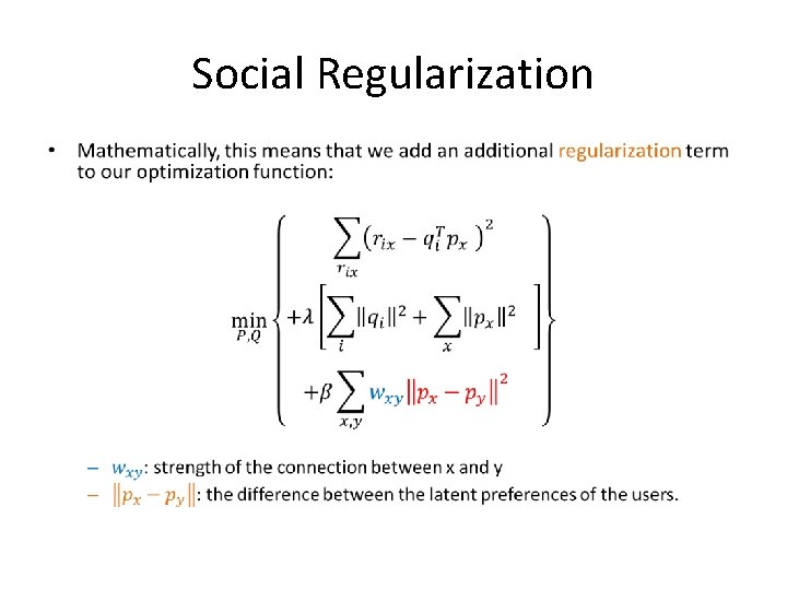
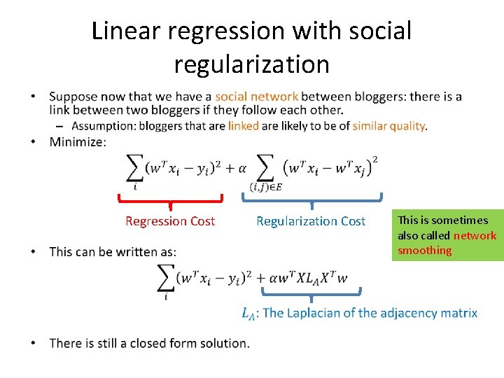
Social Regularization •

Social Regularization • Helps in giving additional information about the preferences of the users • Helps with sparse data since it allows us to make inferences for users for whom we have little data. • The same idea can be applied in different settings

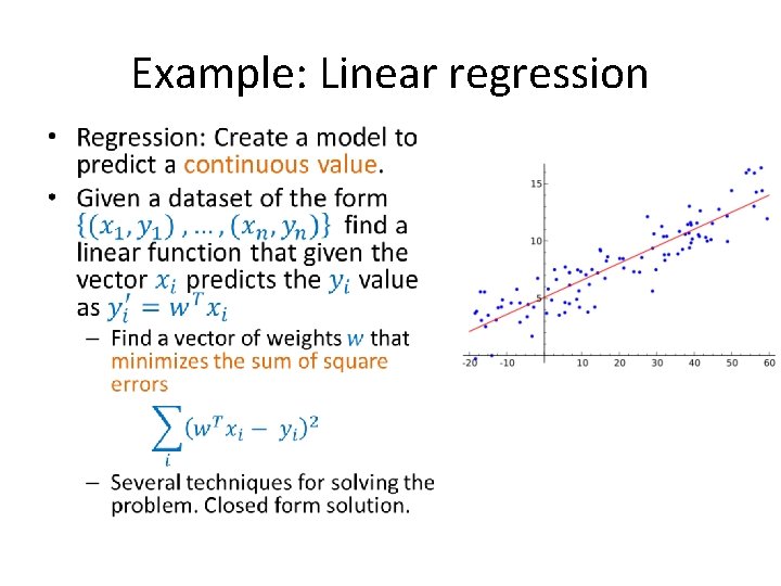
Example: Linear regression •

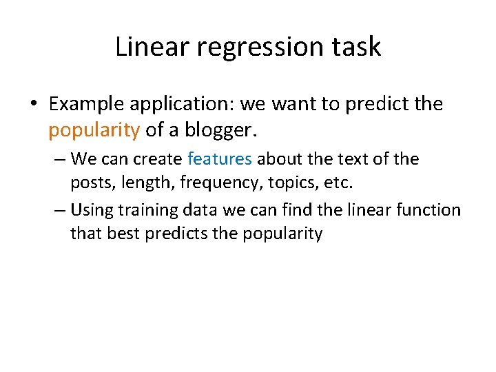
Linear regression task • Example application: we want to predict the popularity of a blogger. – We can create features about the text of the posts, length, frequency, topics, etc. – Using training data we can find the linear function that best predicts the popularity

Linear regression with social regularization • Regression Cost Regularization Cost This is sometimes also called network smoothing

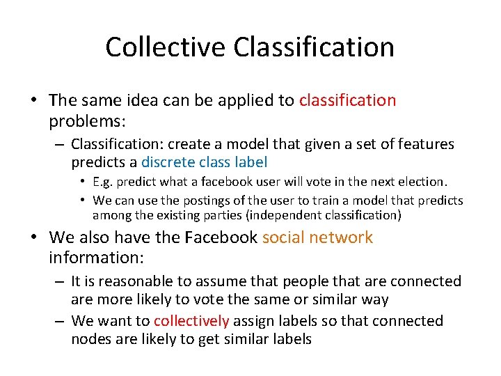
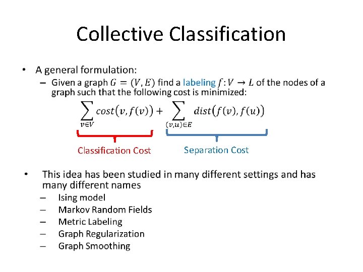
Collective Classification • The same idea can be applied to classification problems: – Classification: create a model that given a set of features predicts a discrete class label • E. g. predict what a facebook user will vote in the next election. • We can use the postings of the user to train a model that predicts among the existing parties (independent classification) • We also have the Facebook social network information: – It is reasonable to assume that people that are connected are more likely to vote the same or similar way – We want to collectively assign labels so that connected nodes are likely to get similar labels

Collective Classification • Classification Cost Separation Cost

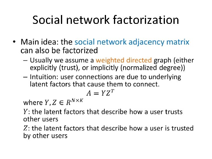
Social network factorization •

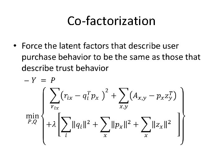
Co-factorization •