Neural Networks Backprop Modular Design Radu Ionescu Prof

Neural Networks. Backprop. Modular Design Radu Ionescu, Prof. Ph. D. raducu. ionescu@gmail. com Faculty of Mathematics and Computer Science University of Bucharest

Plan for Today • Notation + Setup • Neural Networks • Chain Rule + Backprop
 • Output: y (spam or non-spam…)")
Supervised Learning • Input: x (images, text, emails…) • Output: y (spam or non-spam…) • (Unknown) Target Function – f: X Y (the “true” mapping / reality) • Data – (x 1, y 1), (x 2, y 2), …, (x. N, y. N) • Model / Hypothesis Class – g: X Y – y = g(x) = sign(w. Tx) • Learning = Search in hypothesis space – Find best g in model class

Basic Steps of Supervised Learning • Set up a supervised learning problem • Data collection – Start with training data for which we know the correct outcome provided by a teacher or oracle. • Representation – Choose how to represent the data. • Modeling – Choose a hypothesis class: H = {g: X Y} • Learning/Estimation – Find best hypothesis you can in the chosen class. • Model Selection – Try different models. Picks the best one. (More on this later) • If happy, stop – Else refine or more of the above

Error Decomposition Reality r model class n tio a tim r Es Erro Op tim Er izat ro ion r M g lin e od ro Er

Error Decomposition Reality r ng eli d o M O de lc las s n tio iza im or pt Err mo n tio a tim Es Error ro Er

Error Decomposition r model class Higher-Order Potentials n io t a im ror t Es Er O pt im Er iza ro tio r n M eli d o ng ro Er Reality

Biological Neuron

The Neuron Metaphor • Neurons • accept information from multiple inputs • transmit information to other neurons • Artificial neuron • multiply inputs by weights along edges • apply some function to the set of inputs at each node

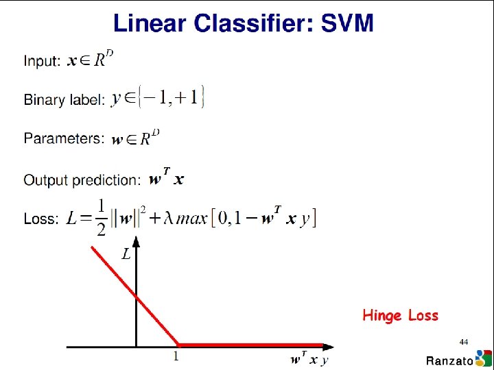
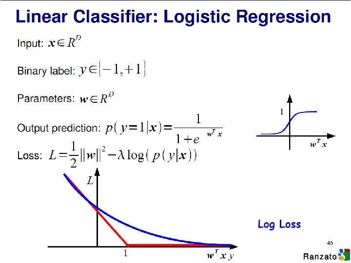
Types of Neurons Linear Neuron Logistic Neuron Potentially more. Require a convex Perceptron loss function for gradient descent training.

Activation Functions • sigmoid vs tanh - saturated gradients towards +/- infinity - sigmoid has non-zero mean
![Rectified Linear Units (Re. LU) [Krizhevsky et al. , NIPS 12]](http://slidetodoc.com/presentation_image_h2/c8822098b439def25680f8a619e1679e/image-12.jpg "Rectified Linear Units (Re. LU) [Krizhevsky et al. , NIPS 12]")
Rectified Linear Units (Re. LU) [Krizhevsky et al. , NIPS 12]

Limitation • A single “neuron” is still a linear decision boundary • What to do? • Idea: Stack a bunch of them together!

Multilayer Networks • Cascade neurons together • The output from one layer is the input to the next • Each layer has its own sets of weights

Multilayer Networks • A 2 -layer neural network: • A 3 -layer neural network:

Detailed architecture of a neural network w 1, 1 xi, 1 w 2, 1 w 1, 1 w 3, 1 b 1, 1=0 w 2, 1 xi, 2 xi, 3 y b 1, 1=0 w 2, 4 w 3, 1 w 4, 1 w 1, 4 b 1, 1=0 w 3, 4 w 1, 1 w 1, 2 w 1, 3 w 1, 4 W 0 = w 2, 1 w 2, 2 w 2, 3 w 2, 4 w 3, 1 w 3, 2 w 3, 3 w 3, 4 W 1 = b 1, 1=0 w 2, 1 w 3, 1 w 4, 1

Limitation • A single “neuron” is still a linear decision boundary • What to do? • Idea: Stack a bunch of them together! • Non-linearities are mandatory (see proof)

Universal Function Approximators • Theorem: A two-layer network with linear outputs can uniformly approximate any continuous function on a finite subset to arbitrary accuracy, given enough hidden units [Funahashi ’ 89]

Visualizing Loss Functions • Sum of individual losses

Detour

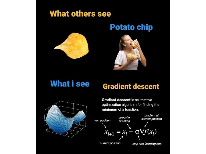
Gradient Descent Algorithm

Gradient Descent Algorithm • In 1 -dimension, the derivative of a function: • In multiple dimensions, the gradient is the vector of partial derivatives.

current W: gradient d. W: [0. 34, -1. 11, 0. 78, 0. 12, 0. 55, 2. 81, -3. 1, -1. 5, 0. 33, …] loss 1. 25347 [? , ? , ? , …]
: gradient d. W: [0. 34, -1. 11,")
current W: W + h (first dim): gradient d. W: [0. 34, -1. 11, 0. 78, 0. 12, 0. 55, 2. 81, -3. 1, -1. 5, 0. 33, …] loss 1. 25347 [0. 34 + 0. 0001, -1. 11, 0. 78, 0. 12, 0. 55, 2. 81, -3. 1, -1. 5, 0. 33, …] loss 1. 25322 [? , ? , ? , …]
: [0. 34, -1. 11, 0. 78, 0.")
current W: W + h (first dim): [0. 34, -1. 11, 0. 78, 0. 12, 0. 55, 2. 81, -3. 1, -1. 5, 0. 33, …] loss 1. 25347 [0. 34 + 0. 0001, -1. 11, 0. 78, 0. 12, 0. 55, 2. 81, -3. 1, -1. 5, 0. 33, …] loss 1. 25322 gradient d. W: [-2. 5, ? , ? , (1. 25322 - 1. 25347)/0. 0001 = -2. 5 ? , ? , ? , …]
: gradient d. W: [0. 34, -1. 11,")
current W: W + h (second dim): gradient d. W: [0. 34, -1. 11, 0. 78, 0. 12, 0. 55, 2. 81, -3. 1, -1. 5, 0. 33, …] loss 1. 25347 [0. 34, -1. 11 + 0. 0001, 0. 78, 0. 12, 0. 55, 2. 81, -3. 1, -1. 5, 0. 33, …] loss 1. 25353 [-2. 5, ? , ? , …]
: [0. 34, -1. 11, 0. 78, 0.")
current W: W + h (second dim): [0. 34, -1. 11, 0. 78, 0. 12, 0. 55, 2. 81, -3. 1, -1. 5, 0. 33, …] loss 1. 25347 [0. 34, -1. 11 + 0. 0001, 0. 78, 0. 12, 0. 55, 2. 81, -3. 1, -1. 5, 0. 33, …] loss 1. 25353 gradient d. W: [-2. 5, 0. 6, ? , (1. 25353 - 1. 25347)/0. 0001 ? , = 0. 6? , ? , …]
: gradient d. W: [0. 34, -1. 11,")
current W: W + h (third dim): gradient d. W: [0. 34, -1. 11, 0. 78, 0. 12, 0. 55, 2. 81, -3. 1, -1. 5, 0. 33, …] loss 1. 25347 [0. 34, -1. 11, 0. 78 + 0. 0001, 0. 12, 0. 55, 2. 81, -3. 1, -1. 5, 0. 33, …] loss 1. 25347 [-2. 5, 0. 6, ? , ? , …]
: [0. 34, -1. 11, 0. 78, 0.")
current W: W + h (third dim): [0. 34, -1. 11, 0. 78, 0. 12, 0. 55, 2. 81, -3. 1, -1. 5, 0. 33, …] loss 1. 25347 [0. 34, -1. 11, 0. 78 + 0. 0001, 0. 12, 0. 55, 2. 81, -3. 1, -1. 5, 0. 33, …] loss 1. 25347 gradient d. W: [-2. 5, 0. 6, 0, ? , (1. 25347 - 1. 25347)/0. 0001 = 0? , ? , …]
 Numerical approach • We choose a small positive h and apply")
Gradient Evaluation 1) Numerical approach • We choose a small positive h and apply the formula: - We obtain an approximate value - Very slow to compute 2) Analytic approach • We use calculus to determine the gradient’s formula as a function of X and W

current W: gradient d. W: [0. 34, -1. 11, 0. 78, 0. 12, 0. 55, 2. 81, -3. 1, -1. 5, 0. 33, …] loss 1. 25347 [-2. 5, 0. 6, 0, 0. 2, 0. 7, -0. 5, 1. 1, 1. 3, -2. 1, …] d. W =. . . (some function of x and W)
 def f(x): y = 0. 5 * (x**4) * 2 -")
Gradient Evaluation (Python) def f(x): y = 0. 5 * (x**4) * 2 - (x**2) + x + 5 return y # 1) Numerical Method h = 0. 001 gradient = (f(x + h) - f(x)) / h # 2) Analythic Method def f_prime(x): y_prime * 2 = (x**3) * 4 - x + 1 return y_prime gradient = f_prime(x)
 def GD(W 0, X, goal, learning. Rate): perf. Goal. Not. Met")
Gradient Descent (Python) def GD(W 0, X, goal, learning. Rate): perf. Goal. Not. Met = true W = W 0 while perf. Goal. Not. Met: gradient = eval_gradient(X, W) W_old = W W = W – learning. Rate * gradient perf. Goal. Not. Met = sum(abs(W - W_old)) > goal
 • Only use")
Mini-batch Gradient Descent • Also known as Stochastic Gradient Descent (SGD) • Only use a small portion of the training set to compute the gradient: . . . while perf. Goal. Not. Met: X_batch = select_random_subsample(X) gradient = eval_gradient(@loss, X_batch, W). . . • Common mini-batch sizes are 32/64/128 examples, e. g. Krizhevsky’s ILSVRC Conv. Net used 256 examples

Logistic Regression as a Cascade Given a library of simple functions Compose into a complicate function

Logistic Regression as a Cascade Given a library of simple functions Compose into a complicate function

Chain Rule

Chain Rule

Chain Rule: All local

Logistic Regression as a Cascade

Logistic Regression as a Cascade

Logistic Regression as a Cascade

Key Computation: Forward-Prop

Key Computation: Back-Prop
![Neural Network Training • Step 1: Compute Loss on mini-batch [F-Pass]](http://slidetodoc.com/presentation_image_h2/c8822098b439def25680f8a619e1679e/image-48.jpg "Neural Network Training • Step 1: Compute Loss on mini-batch [F-Pass]")
Neural Network Training • Step 1: Compute Loss on mini-batch [F-Pass]
![Neural Network Training • Step 1: Compute Loss on mini-batch [F-Pass]](http://slidetodoc.com/presentation_image_h2/c8822098b439def25680f8a619e1679e/image-49.jpg "Neural Network Training • Step 1: Compute Loss on mini-batch [F-Pass]")
Neural Network Training • Step 1: Compute Loss on mini-batch [F-Pass]
![Neural Network Training • Step 1: Compute Loss on mini-batch [F-Pass]](http://slidetodoc.com/presentation_image_h2/c8822098b439def25680f8a619e1679e/image-50.jpg "Neural Network Training • Step 1: Compute Loss on mini-batch [F-Pass]")
Neural Network Training • Step 1: Compute Loss on mini-batch [F-Pass]
![Neural Network Training • Step 1: Compute Loss on mini-batch [F-Pass] • Step 2:](http://slidetodoc.com/presentation_image_h2/c8822098b439def25680f8a619e1679e/image-51.jpg "Neural Network Training • Step 1: Compute Loss on mini-batch [F-Pass] • Step 2:")
Neural Network Training • Step 1: Compute Loss on mini-batch [F-Pass] • Step 2: Compute gradients w. r. t. parameters [B-Pass]
![Neural Network Training • Step 1: Compute Loss on mini-batch [F-Pass] • Step 2:](http://slidetodoc.com/presentation_image_h2/c8822098b439def25680f8a619e1679e/image-52.jpg "Neural Network Training • Step 1: Compute Loss on mini-batch [F-Pass] • Step 2:")
Neural Network Training • Step 1: Compute Loss on mini-batch [F-Pass] • Step 2: Compute gradients w. r. t. parameters [B-Pass]
![Neural Network Training • Step 1: Compute Loss on mini-batch [F-Pass] • Step 2:](http://slidetodoc.com/presentation_image_h2/c8822098b439def25680f8a619e1679e/image-53.jpg "Neural Network Training • Step 1: Compute Loss on mini-batch [F-Pass] • Step 2:")
Neural Network Training • Step 1: Compute Loss on mini-batch [F-Pass] • Step 2: Compute gradients w. r. t. parameters [B-Pass]
![Neural Network Training • Step 1: Compute Loss on mini-batch [F-Pass] • Step 2:](http://slidetodoc.com/presentation_image_h2/c8822098b439def25680f8a619e1679e/image-54.jpg "Neural Network Training • Step 1: Compute Loss on mini-batch [F-Pass] • Step 2:")
Neural Network Training • Step 1: Compute Loss on mini-batch [F-Pass] • Step 2: Compute gradients w. r. t. parameters [B-Pass] • Step 3: Use gradient to update parameters
![Neural Network Training • Step 1: Compute Loss on mini-batch [F-Pass] • Step 2:](http://slidetodoc.com/presentation_image_h2/c8822098b439def25680f8a619e1679e/image-55.jpg "Neural Network Training • Step 1: Compute Loss on mini-batch [F-Pass] • Step 2:")
Neural Network Training • Step 1: Compute Loss on mini-batch [F-Pass] • Step 2: Compute gradients w. r. t. parameters [B-Pass] • Step 3: Use gradient to update parameters - with momentum
 Negative direction of the gradient W 1")
W 2 W(current) Negative direction of the gradient W 1

Equivalent Representations

Backward Propagation Question: Does BPROP work with sigmoid activations only? Answer: Nope, any almost everywhere differentiable transformation works. Question: What is the computational cost of BPROP? Answer: About twice FPROP (need to compute gradients w. r. t. input and parameters at every layer). Note: FPROP and BPROP are dual of each other. E. g. : COPY SUM FPROP BPROP + +
- Slides: 58