Decision Trees Random Forests Radu Ionescu Prof Ph



- Slides: 74

Decision Trees. Random Forests. Radu Ionescu, Prof. Ph. D. raducu. ionescu@gmail. com Faculty of Mathematics and Computer Science University of Bucharest

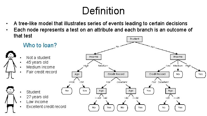
Definition • • A tree-like model that illustrates series of events leading to certain decisions Each node represents a test on an attribute and each branch is an outcome of that test Who to loan? • • Not a student 45 years old Medium income Fair credit record • • Student 27 years old Low income Excellent credit record

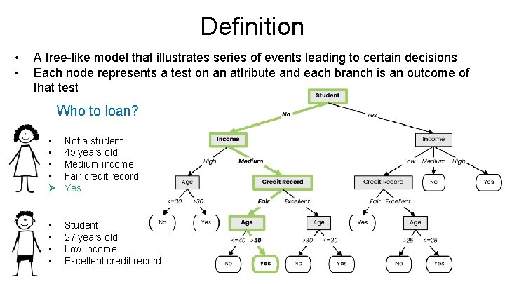
Definition • • A tree-like model that illustrates series of events leading to certain decisions Each node represents a test on an attribute and each branch is an outcome of that test Who to loan? • • Ø Not a student 45 years old Medium income Fair credit record Yes • • Student 27 years old Low income Excellent credit record

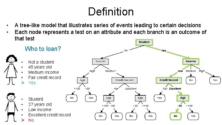
Definition • • A tree-like model that illustrates series of events leading to certain decisions Each node represents a test on an attribute and each branch is an outcome of that test Who to loan? • • Ø Not a student 45 years old Medium income Fair credit record Yes • • Ø Student 27 years old Low income Excellent credit record No

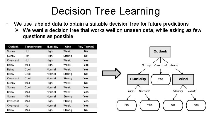
Decision Tree Learning • We use labeled data to obtain a suitable decision tree for future predictions Ø We want a decision tree that works well on unseen data, while asking as few questions as possible

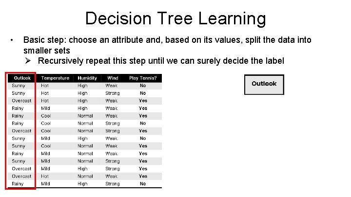
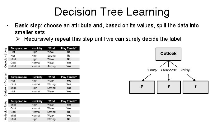
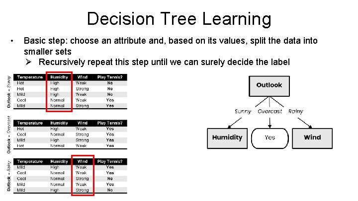
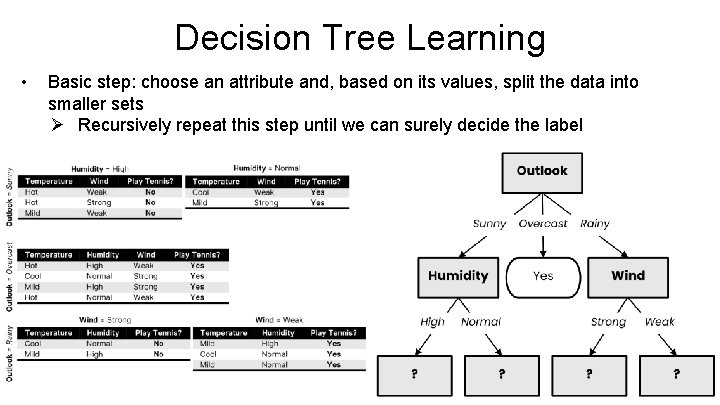
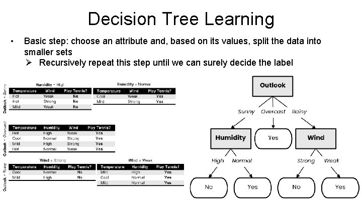
Decision Tree Learning • Basic step: choose an attribute and, based on its values, split the data into smaller sets Ø Recursively repeat this step until we can surely decide the label

Decision Tree Learning • Basic step: choose an attribute and, based on its values, split the data into smaller sets Ø Recursively repeat this step until we can surely decide the label

Decision Tree Learning • Basic step: choose an attribute and, based on its values, split the data into smaller sets Ø Recursively repeat this step until we can surely decide the label

Decision Tree Learning • Basic step: choose an attribute and, based on its values, split the data into smaller sets Ø Recursively repeat this step until we can surely decide the label

Decision Tree Learning • Basic step: choose an attribute and, based on its values, split the data into smaller sets Ø Recursively repeat this step until we can surely decide the label

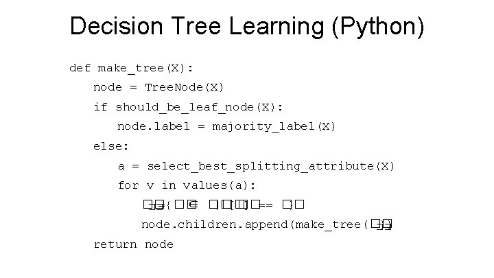
Decision Tree Learning (Python) def make_tree(X): node = Tree. Node(X) if should_be_leaf_node(X): node. label = majority_label(X) else: a = select_best_splitting_attribute(X) for v in values(a): �� ={�� ∈ �� |�� [ �� ] == �� } �� node. children. append(make_tree(�� )) �� return node

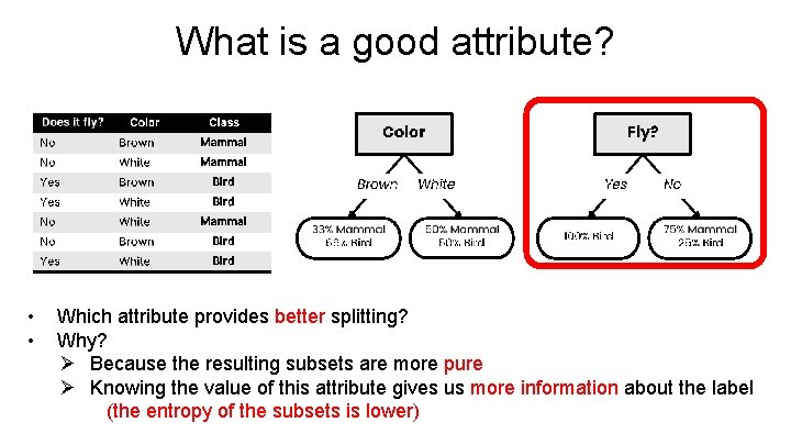
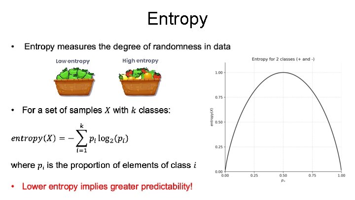
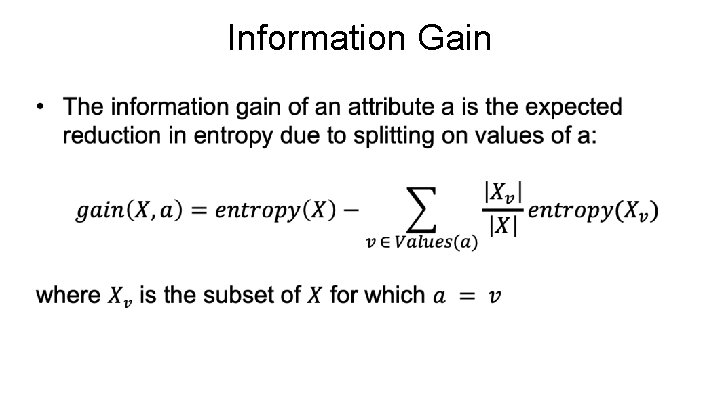
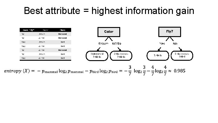
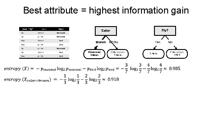
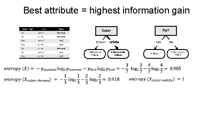
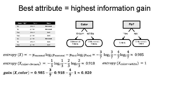
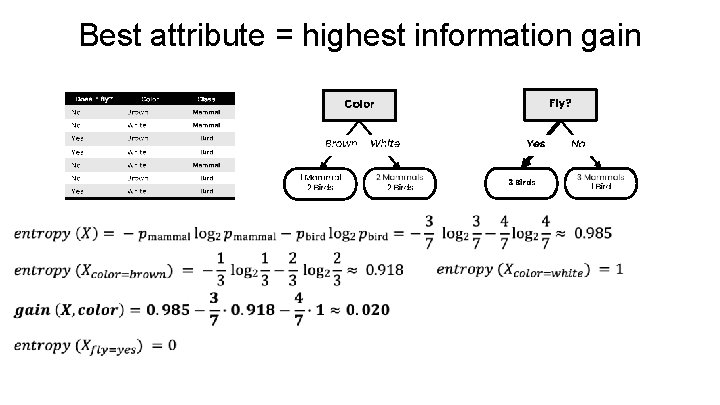
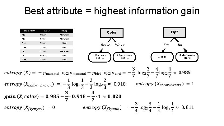
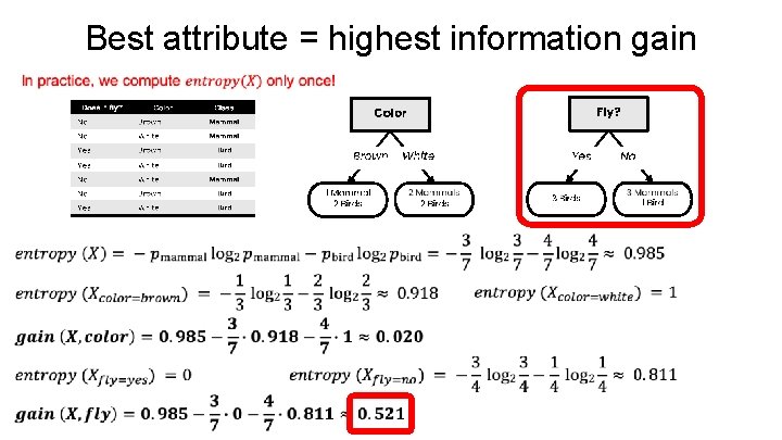
What is a good attribute? • • Which attribute provides better splitting? Why? Ø Because the resulting subsets are more pure Ø Knowing the value of this attribute gives us more information about the label (the entropy of the subsets is lower)

Information Gain

Entropy

Information Gain

Best attribute = highest information gain

Best attribute = highest information gain

Best attribute = highest information gain

Best attribute = highest information gain

Best attribute = highest information gain

Best attribute = highest information gain

Best attribute = highest information gain

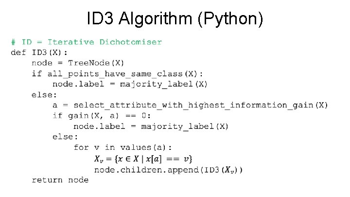
ID 3 Algorithm (Python)

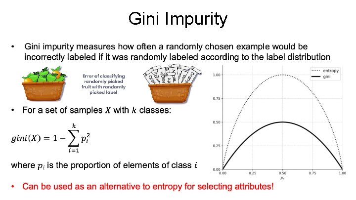
Gini Impurity

Gini Impurity

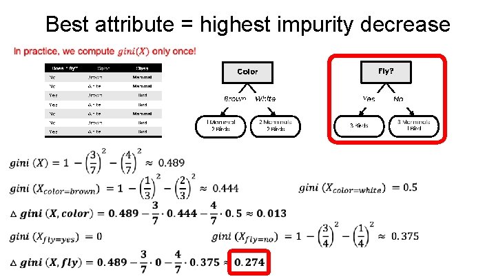
Best attribute = highest impurity decrease

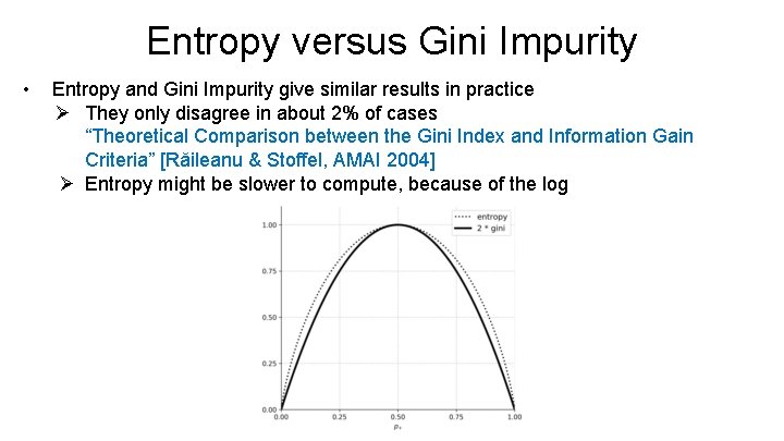
Entropy versus Gini Impurity • Entropy and Gini Impurity give similar results in practice Ø They only disagree in about 2% of cases “Theoretical Comparison between the Gini Index and Information Gain Criteria” [Răileanu & Stoffel, AMAI 2004] Ø Entropy might be slower to compute, because of the log

Pruning

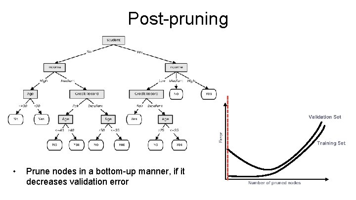
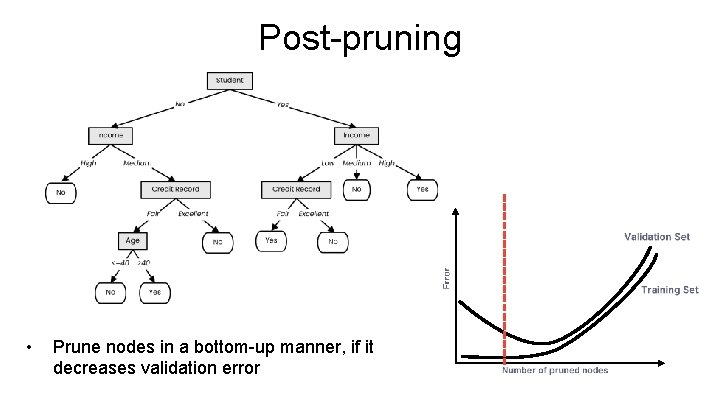
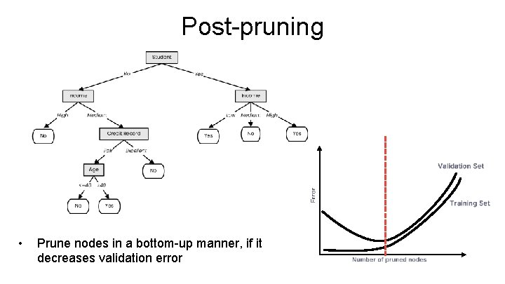
Pruning • Pruning is a technique that reduces the size of a decision tree by removing branches of the tree which provide little predictive power • It is a regularization method that reduces the complexity of the final model, thus reducing overfitting Ø Decision trees are prone to overfitting! • Pruning methods: Ø Pre-pruning: Stop the tree building algorithm before it fully classifies the data Ø Post-pruning: Build the complete tree, then replace some nonleaf nodes with leaf nodes if this improves validation error

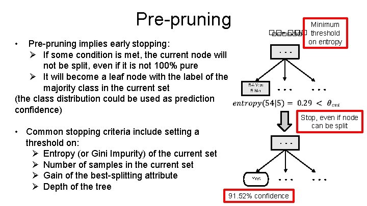
Pre-pruning • Pre-pruning implies early stopping: Ø If some condition is met, the current node will not be split, even if it is not 100% pure Ø It will become a leaf node with the label of the majority class in the current set (the class distribution could be used as prediction confidence) Minimum �� = ��. �� threshold ������ on entropy • Common stopping criteria include setting a threshold on: Ø Entropy (or Gini Impurity) of the current set Ø Number of samples in the current set Ø Gain of the best-splitting attribute Ø Depth of the tree 91. 52% confidence Stop, even if node can be split

Post-pruning • Prune nodes in a bottom-up manner, if it decreases validation error

Post-pruning • Prune nodes in a bottom-up manner, if it decreases validation error

Post-pruning • Prune nodes in a bottom-up manner, if it decreases validation error

Handling Numerical Attributes

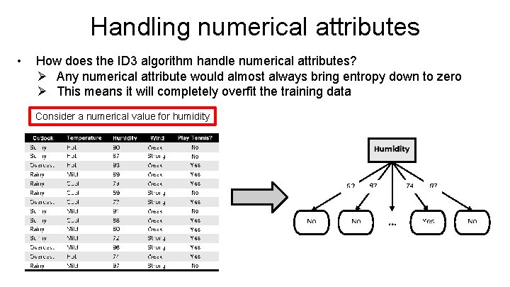
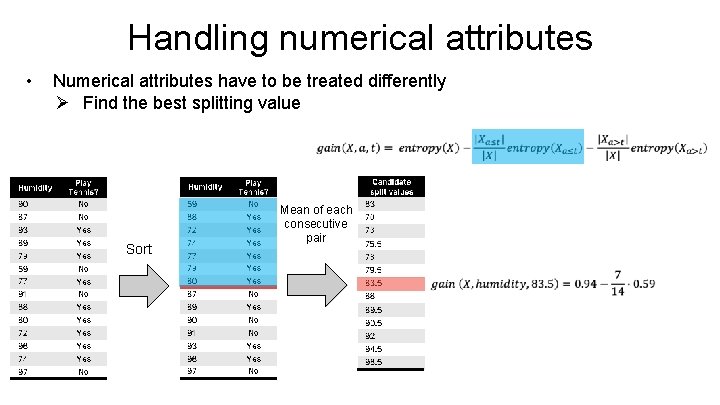
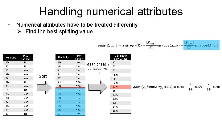
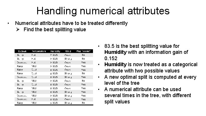
Handling numerical attributes • How does the ID 3 algorithm handle numerical attributes? Ø Any numerical attribute would almost always bring entropy down to zero Ø This means it will completely overfit the training data Consider a numerical value for humidity

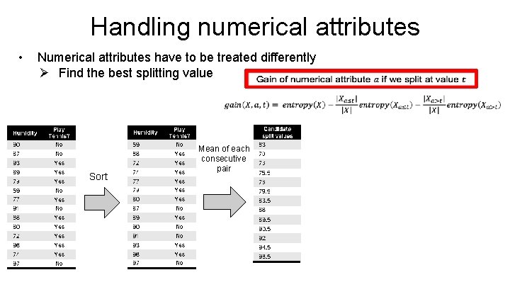
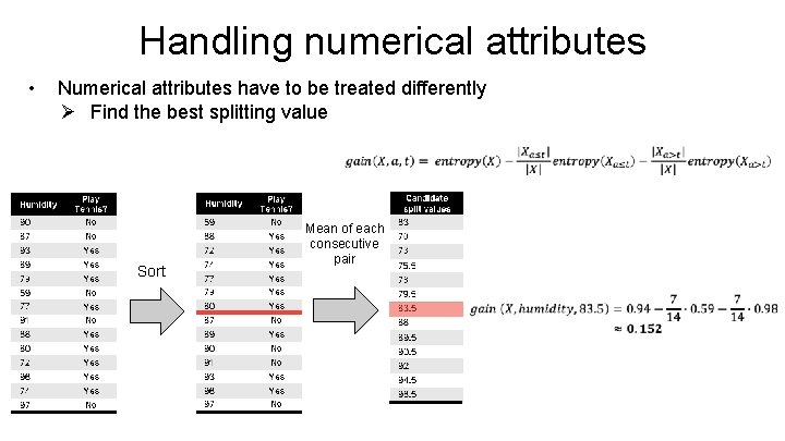
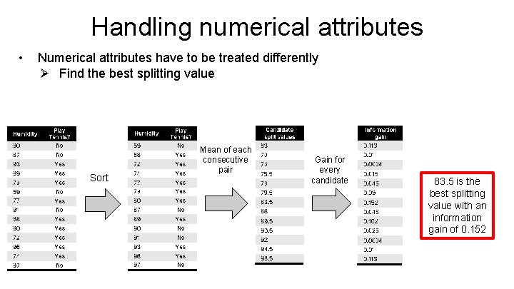
Handling numerical attributes • Numerical attributes have to be treated differently Ø Find the best splitting value Sort Mean of each consecutive pair

Handling numerical attributes • Numerical attributes have to be treated differently Ø Find the best splitting value Sort Mean of each consecutive pair

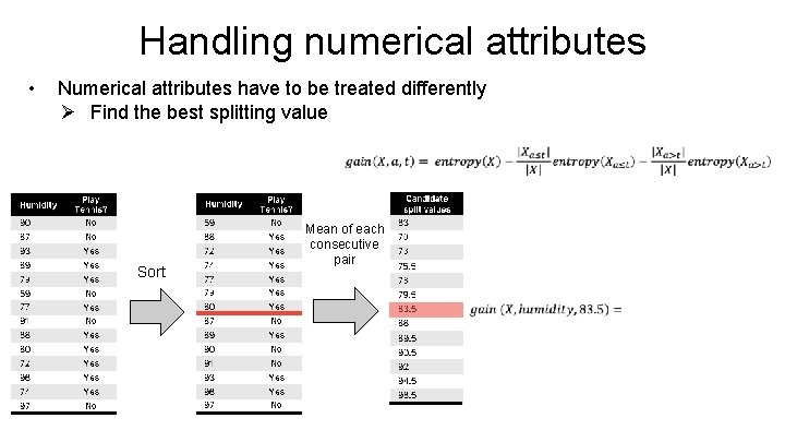
Handling numerical attributes • Numerical attributes have to be treated differently Ø Find the best splitting value Sort Mean of each consecutive pair

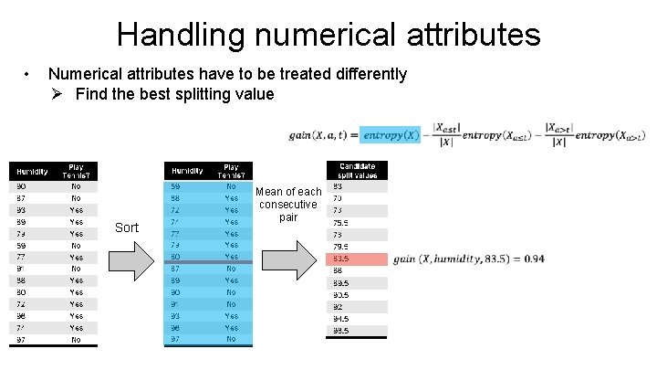
Handling numerical attributes • Numerical attributes have to be treated differently Ø Find the best splitting value Sort Mean of each consecutive pair

Handling numerical attributes • Numerical attributes have to be treated differently Ø Find the best splitting value Sort Mean of each consecutive pair

Handling numerical attributes • Numerical attributes have to be treated differently Ø Find the best splitting value Sort Mean of each consecutive pair

Handling numerical attributes • Numerical attributes have to be treated differently Ø Find the best splitting value Sort Mean of each consecutive pair Gain for every candidate 83. 5 is the best splitting value with an information gain of 0. 152

Handling numerical attributes • Numerical attributes have to be treated differently Ø Find the best splitting value > > ≤ ≤ ≤ > ≤ > • 83. 5 is the best splitting value for Humidity with an information gain of 0. 152 • Humidity is now treated as a categorical attribute with two possible values • A new optimal split is computed at every level of the tree • A numerical attribute can be used several times in the tree, with different split values

Handling Missing Values

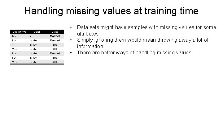
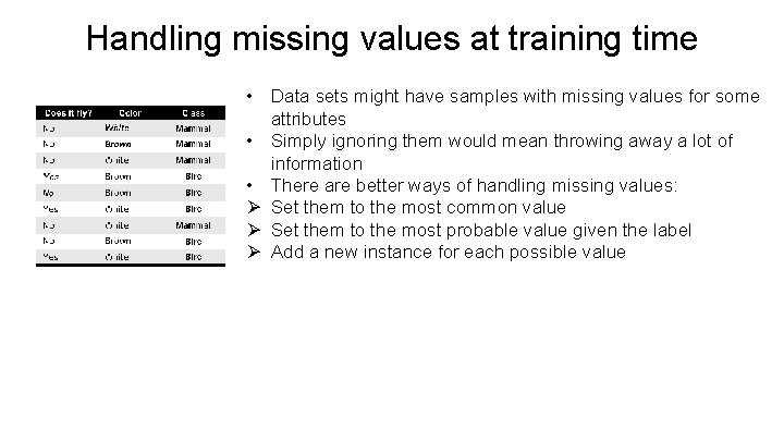
Handling missing values at training time • Data sets might have samples with missing values for some attributes • Simply ignoring them would mean throwing away a lot of information • There are better ways of handling missing values:

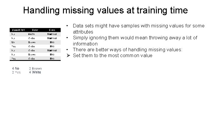
Handling missing values at training time • Data sets might have samples with missing values for some attributes • Simply ignoring them would mean throwing away a lot of information • There are better ways of handling missing values: Ø Set them to the most common value

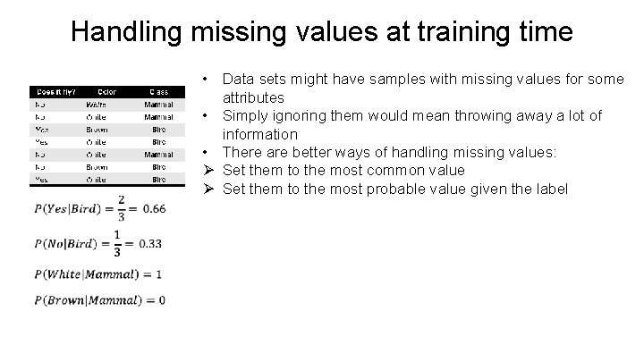
Handling missing values at training time • Data sets might have samples with missing values for some attributes • Simply ignoring them would mean throwing away a lot of information • There are better ways of handling missing values: Ø Set them to the most common value Ø Set them to the most probable value given the label

Handling missing values at training time • Data sets might have samples with missing values for some attributes • Simply ignoring them would mean throwing away a lot of information • There are better ways of handling missing values: Ø Set them to the most common value Ø Set them to the most probable value given the label Ø Add a new instance for each possible value

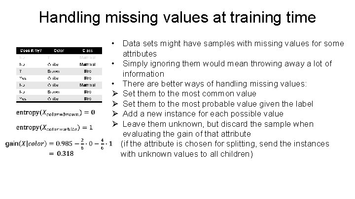
Handling missing values at training time • Data sets might have samples with missing values for some attributes • Simply ignoring them would mean throwing away a lot of information • There are better ways of handling missing values: Ø Set them to the most common value Ø Set them to the most probable value given the label Ø Add a new instance for each possible value Ø Leave them unknown, but discard the sample when evaluating the gain of that attribute (if the attribute is chosen for splitting, send the instances with unknown values to all children)

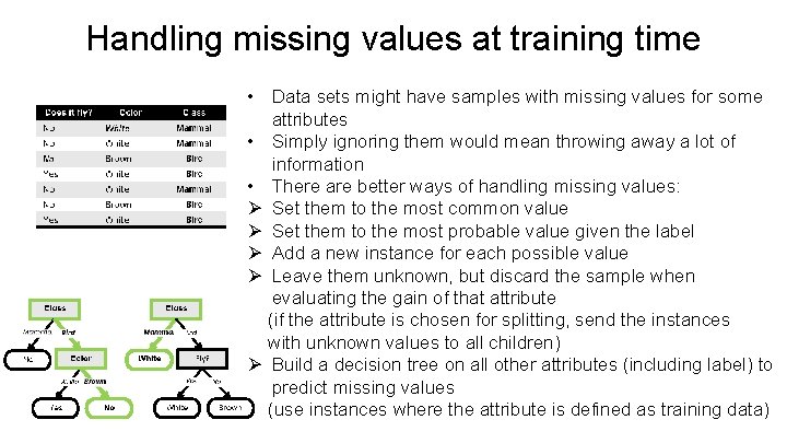
Handling missing values at training time • Data sets might have samples with missing values for some attributes • Simply ignoring them would mean throwing away a lot of information • There are better ways of handling missing values: Ø Set them to the most common value Ø Set them to the most probable value given the label Ø Add a new instance for each possible value Ø Leave them unknown, but discard the sample when evaluating the gain of that attribute (if the attribute is chosen for splitting, send the instances with unknown values to all children) Ø Build a decision tree on all other attributes (including label) to predict missing values (use instances where the attribute is defined as training data)

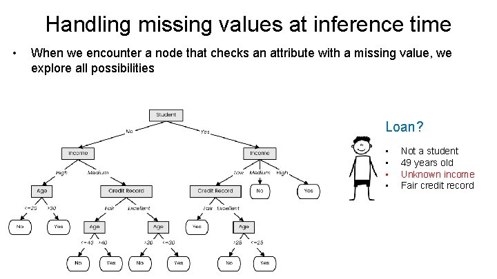
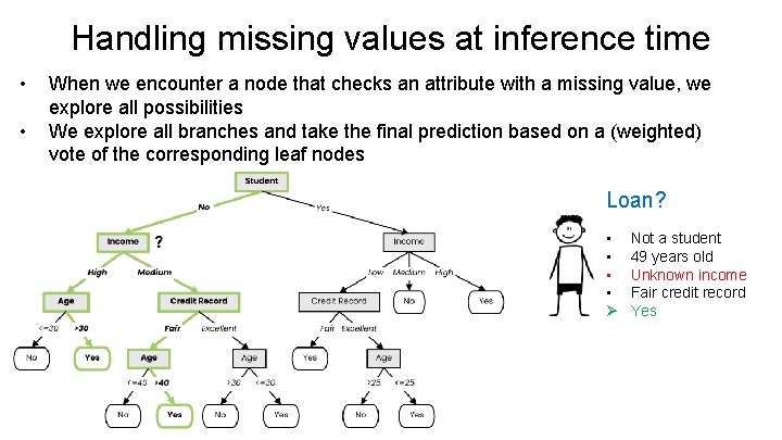
Handling missing values at inference time • When we encounter a node that checks an attribute with a missing value, we explore all possibilities Loan? • • Not a student 49 years old Unknown income Fair credit record

Handling missing values at inference time • • When we encounter a node that checks an attribute with a missing value, we explore all possibilities We explore all branches and take the final prediction based on a (weighted) vote of the corresponding leaf nodes Loan? • • Ø Not a student 49 years old Unknown income Fair credit record Yes

C 4. 5 Algorithm • C 4. 5 algorithm is an extension of ID 3 algorithm that brings several improvements: Ø Ability to handle both categorical (discrete) and numerical (continuous) attributes (continuous attributes are split by finding a best-splitting threshold) Ø Ability to handle missing values both at training and inference time (missing values at training are not used when information gain is computed; missing values at inference time are handled by exploring all corresponding branches) Ø Ability to handle attributes with different costs Ø Post-pruning in a bottom-up manner for removing branches that decrease validation error (i. e. , that increase generalization capacity)

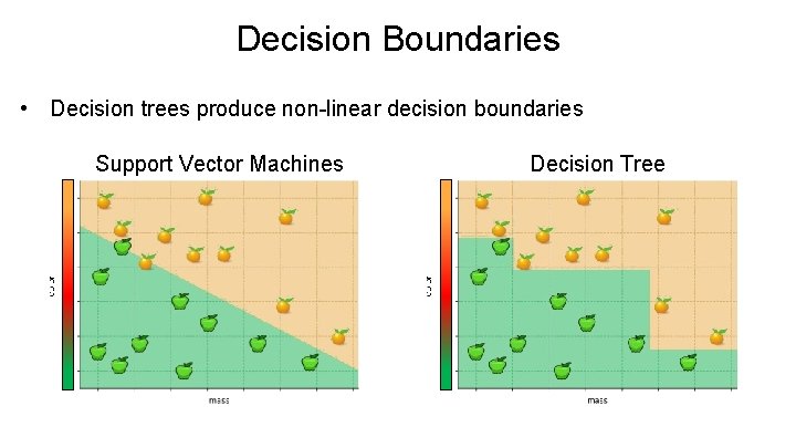
Decision Boundaries • Decision trees produce non-linear decision boundaries Support Vector Machines Decision Tree

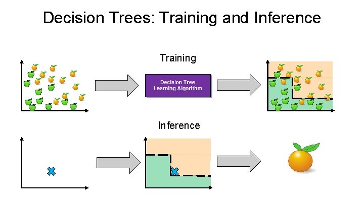
Decision Trees: Training and Inference Training Inference

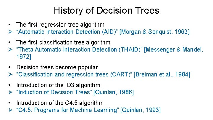
History of Decision Trees • The first regression tree algorithm Ø “Automatic Interaction Detection (AID)” [Morgan & Sonquist, 1963] • The first classification tree algorithm Ø “Theta Automatic Interaction Detection (THAID)” [Messenger & Mandel, 1972] • Decision trees become popular Ø “Classification and regression trees (CART)” [Breiman et al. , 1984] • Introduction of the ID 3 algorithm Ø “Induction of Decision Trees” [Quinlan, 1986] • Introduction of the C 4. 5 algorithm Ø “C 4. 5: Programs for Machine Learning” [Quinlan, 1993]

Summary • Decision trees represent a tool based on a tree-like graph of decisions and their possible outcomes • Decision tree learning is a machine learning method that employs a decision tree as a predictive model • ID 3 builds a decision tree by iteratively splitting the data based on the values of an attribute with the largest information gain (decrease in entropy) Ø Using the decrease of Gini Impurity is also a commonly-used option in practice • C 4. 5 is an extension of ID 3 that handles attributes with continuous values, missing values and adds regularization by pruning branches likely to overfit

Random Forests (Ensemble learning with decision trees)

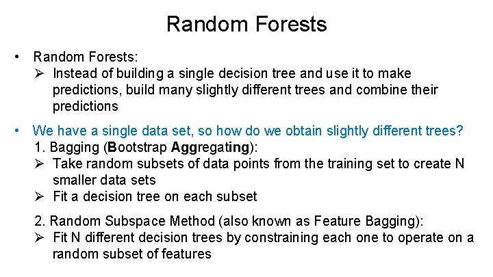
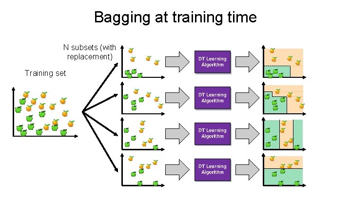
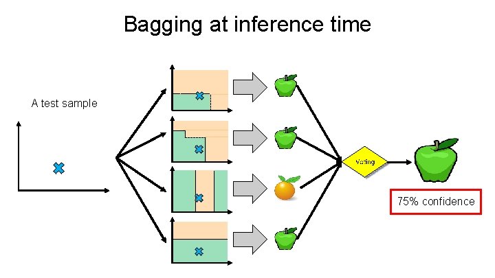
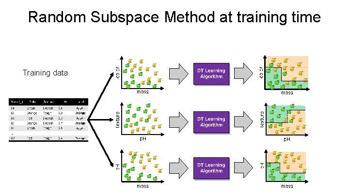
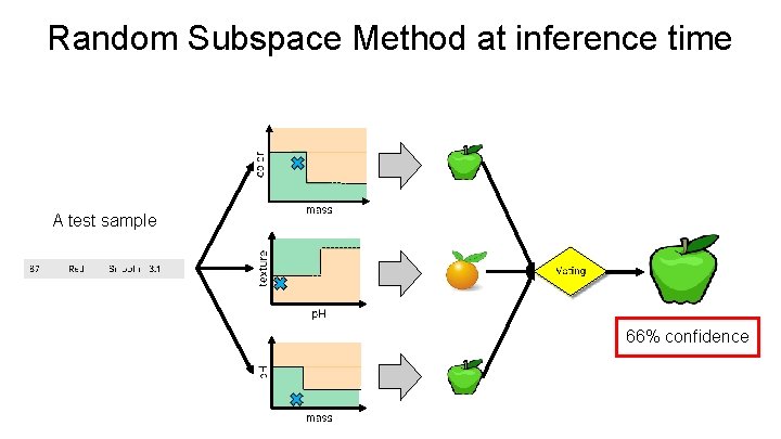
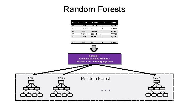
Random Forests • Random Forests: Ø Instead of building a single decision tree and use it to make predictions, build many slightly different trees and combine their predictions • We have a single data set, so how do we obtain slightly different trees? 1. Bagging (Bootstrap Aggregating): Ø Take random subsets of data points from the training set to create N smaller data sets Ø Fit a decision tree on each subset 2. Random Subspace Method (also known as Feature Bagging): Ø Fit N different decision trees by constraining each one to operate on a random subset of features

Bagging at training time N subsets (with replacement) Training set

Bagging at inference time A test sample 75% confidence

Random Subspace Method at training time Training data

Random Subspace Method at inference time A test sample 66% confidence

Random Forests Tree 1 Tree 2 Random Forest Tree N

History of Random Forests • Introduction of the Random Subspace Method Ø “Random Decision Forests” [Ho, 1995] and “The Random Subspace Method for Constructing Decision Forests” [Ho, 1998] • Combined the Random Subspace Method with Bagging. Introduce the term Random Forest (a trademark of Leo Breiman and Adele Cutler) Ø “Random Forests” [Breiman, 2001]

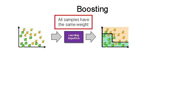
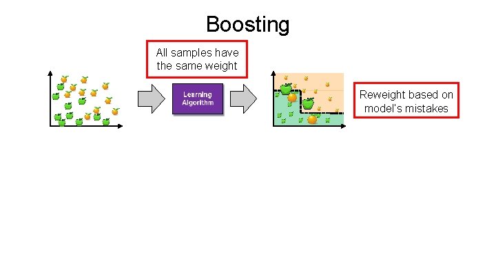
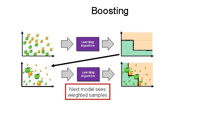
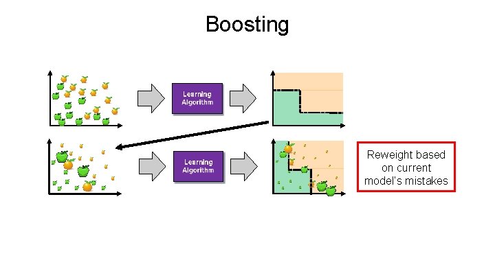
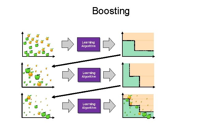
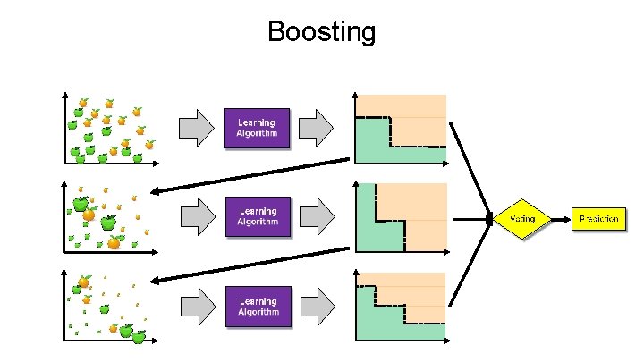
Ensemble Learning • Ensemble Learning: Ø Method that combines multiple learning algorithms to obtain performance improvements over its components • Random Forests are one of the most common examples of ensemble learning • Other commonly-used ensemble methods: Ø Bagging: multiple models on random subsets of data samples Ø Random Subspace Method: multiple models on random subsets of features Ø Boosting: train models iteratively, while making the current model focus on the mistakes of the previous ones by increasing the weight of misclassified samples

Boosting All samples have the same weight

Boosting All samples have the same weight Reweight based on model’s mistakes

Boosting Next model sees weighted samples

Boosting Reweight based on current model’s mistakes

Boosting

Boosting

Summary • Ensemble Learning methods combine multiple learning algorithms to obtain performance improvements over its components • Commonly-used ensemble methods: Ø Bagging (multiple models on random subsets of data samples) Ø Random Subspace Method (multiple models on random subsets of features) Ø Boosting (train models iteratively, while making the current model focus on the mistakes of the previous ones by increasing the weight of misclassified samples) • Random Forests are an ensemble learning method that employ decision tree learning to build multiple trees through bagging and random subspace method. Ø They rectify the overfitting problem of decision trees!

Decision Trees and Random Forest (Python) from sklearn. tree import Decision. Tree. Classifier from sklearn. ensemble import Random. Forest. Classifier clf = Decision. Tree. Classifier(criterion = "entropy", min_samples_leaf = 3) # Lots of parameters: criterion = "gini" / "entropy"; # max_depth; # min_impurity_split; clf. fit(X, y) # It can only handle numerical attributes! # Categorical attributes need to be encoded, see Label. Encoder and One. Hot. Encoder clf. predict([x]) # Predict class for x clf. feature_importances_ # Importance of each feature clf. tree_ # The underlying tree object clf = Random. Forest. Classifier(n_estimators = 20) # Random Forest with 20 trees