Micro Arrays and proteomics Arne Elofsson Introduction Microarrays

Micro. Arrays and proteomics Arne Elofsson

Introduction ● Microarrays – – – ● Proteomics – – – ● Introduction Data threatment Analysis Introduction and methodologis Data threatment Analysis The network view of biology – Connectivity vs function

Topics ● Goal – study many genes at once ● Major types of DNA microarray ● How to roll your own ● Designing the right experiment ● Many pretty spots – Now what? ● Interpreting the data

The Goal “Big Picture” biology – – What are all the components & processes taking place in a cell? – How do these components & processes interact to sustain life? One approach: What happens to the entire cell when one particular gene/process is perturbed?

Genome Sequence Flood ● Typical results from initial analysis of a new genome by the best computational methods: For 1/3 of the genes we have a “good” idea what they are doing (high similarity to exp. studied genes) For 1/3 of the genes, we have a guess at what they are doing (some similarity to previously seen genes) For 1/3 of genes, we have no idea what they are doing (no similarity to studied genes)

Large Scale Approaches ● ● ● Geneticists used to study only one (or a few) genes at a time Now, thousands of identified genes to assign biological function to Microarrays allow massively parallel measurements in one experiment (3 orders of magnitude or greater)

Southern and Northern Blots Basic DNA detection technique that has been used for over 30 years: ● Northern Blots ● Hybridizing labelled DNA to a solid support with RNA from cells. – ● Southern blots: 1. 2. 3. 4. A “known” strand of DNA is deposited on a solid support (i. e. nitrocellulose paper) An “unknown” mixed bag of DNA is labelled (radioactive or fluorescent) “Unknown” DNA solution allowed to mix with known DNA (attached to nitro paper), then excess solution washed off If a copy of “known” DNA occurs in “unknown” sample, it will stick (hybridize), and labeled DNA will be detected on photographic film

The process Building the chip: MASSIVE PCR PURIFICATION AND PREPARATION PREPARING SLIDES RNA preparation: CELL CULTURE AND HARVEST PRINTING Hybridizing the chip: POST PROCESSING ARRAY HYBRIDIZATION RNA ISOLATION c. DNA PRODUCTION PROBE LABELING DATA ANALYSIS

An Array Experiment

The arrayer Ngai Lab arrayer , UC Berkeley Print-tip head

Pins collect c. DNA from wells 384 well plate Print-tip group 1 c. DNA clones Contains c. DNA probes Glass Slide Array of bound c. DNA probes 4 x 4 blocks = 16 print-tip groups Spotted in duplicate Print-tip group 6

Scanning Detector PMT Image Duplicate spots

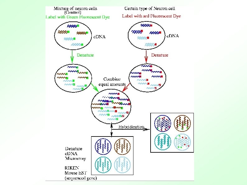
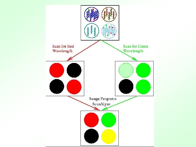
Microarray summary ● ● ● Create 2 ssamples Label one green and one red Mix in equal amounts and hybridze in array Process images and normalize data Read data

RGB overlay of Cy 3 and Cy 5 images

Microarray life cyle Biological Question Data Analysis & Modelling Sample Preparation Microarray. D etection Taken from Schena & Davis Microarray Reaction

Biological question Differentially expressed genes Sample class prediction etc. Experimental design Microarray experiment 16 -bit TIFF files Image analysis (Rfg, Rbg), (Gfg, Gbg) Normalization R, G Estimation Testing Clustering Biological verification and interpretation Discrimination

Yeast Genome Expression Array

Different types of Arrays • Gene Expression arrays • Non gene expression arrays – c. DNA (Brown/Botstein) – CHIP-CHIP ARRAYS • One c. DNA on each spot • immunoprecipitation to micro -arrays that contain genomic • Spotted regions (Ch. IP-chip) has – Affymetrix provided investigators with • Short oligonucleotides the ability to identify, in a • Photolithography high-throughput manner, promoters directly bound by – Ink-jet microarrays from Agilent specific transcription factors. • 25 -60 -mers “printed directly on glass slides – SNPs • Flexible, rapid, but expensive – Genomic (tiling) arrays

Pros/Cons of Different Technologies • • • Spotted Arrays relative cheap to make (~$10 slide) flexible - spot anything you want Cheap so can repeat experiments many times highly variable spot deposition usually have to make your own Accuracy at extremes in range may be less • • • Affymetrix Gene Chips expensive ($500 or more) limited types avail, no chance of specialized chips fewer repeated experiments usually more uniform DNA features Can buy off the shelf Dynamic range may be slightly better

Data processing ● Image analysis ● Normalisation – Log 2 transformation

Image Analysis & Data Visualization Cy 3 Experiments Cy 5 Cy 3 Genes Underexpressed Overexpressed Cy 5 log 2 Cy 3 8 4 2 fold 2 4 8

Why Normalization ? To remove systematic biases, which include, ● Sample preparation ● Variability in hybridization ● Spatial effects ● Scanner settings ● Experimenter bias

What Normalization Is & What It Isn’t ● Methods and Algorithms ● Applied after some Image Analysis ● Applied before subsequent Data Analysis ● Allows comparison of experiments ● Not a cure for poor data.

Where Normalization Fits In Sample Preparation Hybridization Scanning + Image Analysis Normalization Data Analysis Array Fabrication Normalization Spot location, assignment of intensities, background correction etc. Subsequent analysis, e. g clustering, uncovering genetic networks

Choice of Probe Set Normalization method intricately linked to choice of probes used to perform normalization ● House keeping genes – e. g. Actin, GAPDH ● Larger subsets – Rank invariant sets Schadt et al (2001) J. Cellular Biochemistry 37 ● Spiked in Controls ● Chip wide normalization – all spots

Form of Data Working with logged values gives symmetric distribution Global factors such as total m. RNA loading and effect of PMT settings easily eliminated.

Mean & Median Centering ● Simplistic Normalization Procedure ● Assume No overall change in D. E. Mean log (m. RNA ratio) is same between experiments. ● Spot intensity ratios not perfect log(ratio) – mean(log ratio) or log(ratio) – median(log ratio) more robust

Location & Scale Transformations 0 0 Mean & Median centering are examples of location transformations

Regression Methods • Compare two hybridizations (exp. and ref) – use scatter plot • If perfect comparability – straight line through 0, slope 1 • Normalization – fit straight line and adjust to 0 intercept and slope 1 • Various robust procedures exist

M-A Plots M-A plot is 45° rotation of standard scatter plot log R M 45° A log G M = log R – log G A = ½[ log R + log G ] M = Minus A = Add

M-A Plots M M Un-normalized Normalized A Normalized M values are just heights between spots and the “general trend” (red line) A

Methods To Determine General Trend ● Lowess (loess) Y. H. Yang et al, Nucl. Acid. Res. 30 (2002) ● ● Local Average Global Non-linear Parametric Fit e. g. Polynomials Standard Orthogonal decompositions e. g. Fourier Transforms Non-orthogonal decompositions e. g. Wavelets

Lowess Gasch et al. (2000) Mol. Biol. Cell 11, 4241 -4257

Lowess Demo 1 M A

Lowess Demo 2 M A

Lowess Demo 3 M A

Lowess Demo 4 M A

Lowess Demo 5 M A

Lowess Demo 6 M A

Lowess Demo 7 M A

Things You Can Do With Lowess (and other methods) Bias from different sources can be corrected sometimes by using independent variable. ● Correct bias in MA plot for each print-tip ● Correct bias in MA plot for each sector ● Correct bias due to spatial position on chip

Non-Local Intensity Dependent Normalization

Pros & Cons of Lowess ● No assumption of mathematical form – flexible ● Easy to use ● Slow - unless equivalent kernel pre-calculated ● Too flexible ? Parametric forms just as good and faster to fit.

What is BASE? ● Bio. Array Software Environment ● A complete microarray database system – Array printing LIMS – Sample preparation LIMS – Data warehousing – Data filtering and analysis

What is BASE? ● ● Written by Carl Troein et al at Lund University, Sweden Webserver interface, using free (open source and no-cost) software – Linux, Apache, PHP, My. SQL

Why use BASE? ● Intergrated system for microarray data storage and analysis ● MAGE-ML data output ● Sharing of data ● Free ● Regular updates/bug fixes

Features of BASE ● Password protected ● Individual / group / world access to data ● New analysis tools via plugins ● User-defined data output formats

Using BASE ● Annotation ● Array printing LIMS ● Biomaterials ● Hybridization ● Analysis

Annotation ● Reporters – what is printed on array ● Annotation updated monthly ● Corresponds to Clone search data ● Custom fields can be added ● Dynamically linked to array data

Analysis ● Done as ‘experiments’ ● One or more hybridizations per experiment ● Hybridizations treated as ‘bioassays’ ● Pre-select reporters of interest

Analysis II ● Filter data – ● Merge data – ● Intensity, Ratio, Specific reporters etc. Mean values, Fold ratios, Avg A Quality control – Array plots

Analysis III ● Normalization – ● Statistics – ● Global, Print-tip, Between arrays, etc T-test, B-stats, signed rank Clustering, PCA and MDS

MIAMI Minimum Information About a Microarray Experiment ● ● ● Experimental design Array Design Samples Hybridization Measurements Normalization

Mining gene expression data ● Data mining and analysis 1. Data quality checking 2. Data modification 3. Data summary 4. Data dimensionality reduction 5. Feature selection and extraction 6. Clustering Methods

Data mining methods – – Clustering – Unsupervised learning – K-means, Self Organizing Maps etc Classifications – Supervised learning ● ● – Support Vector machines Neural networks Columns or Rows – Related cells or Genes

Clustering – Pattern representation – – Pattern proximity – – Number of genes and experiments How to measure similarity between patterns – Euclidean distance – Manhattan distance – Minkowski distance Pattern Grouping – What groups to join – Similar to phylogeny

Some potential questions when trying to cluster ● ● What uncategorized genes have an expression pattern similar to these genes that are well-characterized? How different is the pattern of expression of gene X from other genes? ● What genes closely share a pattern of expression with gene X? ● What category of function might gene X belong to? ● ● ● What are all the pairs of genes that closely share patterns of expression? Are there subtypes of disease X discernible by tissue gene expression? What tissue is this sample tissue closest to?

Questions – cont. ● ● ● Which are the different patterns of gene expression? Which genes have a pattern that may have been a result of the influence of gene X? What are all the gene-gene interactions present among these tissue samples? Which genes best differentiate these two group of tissues? Which gene-gene interactions best differentiate these two groups of tissue samples. DIFFERENT ALGORITHMS ARE MORE PARTICULARLY SUITED TO ANSWER SOME OF THESE QUESTIONS, COMPARED WITH THE OTHERS.

One example of clustering – One Dissimilarity matrix 1 2 3 4 5 0 1 5 9 8 0 4 8 7 0 3 4 0 2 0

1 Hierarchical clustering 1 2 3 4 5 0 1 5 9 8 0 4 8 7 0 3 4 0 2 2 3 4 5 1. Place each pattern in a separate cluster 2. Compute proximity matrix for all pairs 3. Find the most similar pair of clusters, merge these 4. Update the proximity matrix 5. Go to 2 if more than one cluster 0

Hierarchical clustering 2 1 2 3 4 5 0 1 5 9 8 0 4 8 7 0 3 4 0 2 5 0 Cluster Object 1 and 2 – 1+2 3 4 5 0 4 8 8 0 3 4 0 2 0

Hierarchical clustering 3 1+2 3 4 5 0 4 8 8 0 3 4 0 2 3 4 5 0 Cluster Object 4 and 5 – 1+2 3 5 1+2 3 4+5 0 4 7 0 3 0

Dendrogram

Clustering micro array data – Possible problems – What is the optimal partitioning – Single linkage has chaining effects

Hierarchical Clustering Results • Image source: http: //cfpub. epa. gov/ncer_abstracts/index. cfm/fuseaction/display. abstract. Detail/abstract/975/report/2001

Non-dendritic clustering – Non hierarchical, a single partitioning – Less computationally expensive – A criterion function – – Square error K-means algorithm – Easy to understand – Easy to implement – Good time complexity

K-means 1. Choose K cluster centres randomly 2. Assign each pattern to its closest centre 3. 4. 5. Compute the new cluster centres using the new clusters Repeat until a convergence criteria is obtained Adjust the number of clusters by merging/splitting

Pluses and minuses of k-means ● Pluses: Low complexity ● Minuses – Mean of a cluster may not be easy to define (data with categorical attributes) – Necessity of specifying k – Not suitable for discovering clusters of non-convex shape or of very different sizes – Sensitive to noise and outlier data points (a small number of such data can substantially influence the mean value) – Some of the above objections (especially the last one) can be overcome by the k-medoid algorithm. ● Instead of the mean value of the objects in a cluster as a reference point, the medoid can be used, which is the most centrally located object in a cluster.

Self Organizing maps – – Representing high-dimensionality data in low dimensionality space SOM – – – A set of input nodes V A set of output nodes C A set of weight parameters W A map topology that defines the distances between any two output nodes Each input node is connected to every output node via a variable connection with a weight. For each input vector there is a winner node with the minimum distance to the input node.

Self organizing maps ● ● ● A neural network algorithm that has been used for a wide variety of applications, mostly for engineering problems but also for data analysis. SOM can be used at the same time both to reduce the amount of data by clustering, and for projecting the data nonlinearly onto a lower-dimensional display. SOM vs k-means – In the SOM the distance of each input from all of the reference vectors instead of just the closest one is taken into account, weighted by the neighborhood kernel h. Thus, the SOM functions as a conventional clustering algorithm if the width of the neighborhood kernel is zero. – Whereas in the K-means clustering algorithm the number K of clusters should be chosen according to the number of clusters there are in the data, in the SOM the number of reference vectors can be chosen to be much larger, irrespective of the number of clusters. The cluster structures will become visible on the special displays

SOM algorithm 1. Initialize the topology and output map 2. Initialize the weights with random values 3. Repeat until convergence 1. Present a new input vector 2. Find the winning node 3. Update weights

Kohonen Self Organizing Feature Maps (SOFM) ● ● Creates a map in which similar patterns are plotted next to each other Data visualization technique that reduces n dimensions and displays similarities More complex than k-means or hierarchical clustering, but more meaningful Neural Network Technique – Inspired by the brain From “Data Analysis Tools for DNA Microarrays” by Sorin Draghici

SOFM Description ● ● Each unit of the SOFM has a weighted connection to all inputs Output Layer As the algorithm progresses, neighboring units are grouped by similarity Input Layer From “Data Analysis Tools for DNA Microarrays” by Sorin Draghici

SOFM Algorithm Initialize Map For t from 0 to 1 t is the learning factor Randomly select a sample Get best matching unit Scale neighbors Increase t a small amount decrease learning factor End for From: http: //davis. wpi. edu/~matt/courses/soms/

An Example Using Colour Three dimensional data: red, blue, green Will be converted into 2 D image map with clustering of Dark Blue and Greys together and Yellow close to Both the Red and the Green From http: //davis. wpi. edu/~matt/courses/soms/

An Example Using Color Each color in the map is associated with a weight From http: //davis. wpi. edu/~matt/courses/soms/

An Example Using Color 1. Initialize the weights Random Values Colors in the Corners Equidistant From http: //davis. wpi. edu/~matt/courses/soms/

An Example Using Color Continued 1. Get best matching unit After randomly selecting a sample, go through all weight vectors and calculate the best match (in this case using Euclidian distance) Think of colors as 3 D points each component (red, green, blue) on an axis From http: //davis. wpi. edu/~matt/courses/soms/

An Example Using Color Continued 1. Getting the best matching unit continued… For example, lets say we chose green as the sample. Then it can be shown that light green is closer to green than red: Green: (0, 6, 0) Light Green: (3, 6, 3) Red(6, 0, 0) This step is repeated for entire map, and the weight with the shortest distance is chosen as the best match From http: //davis. wpi. edu/~matt/courses/soms/

An Example Using Color Continued 1. Scale neighbors 1. 2. Determine which weights are considred nieghbors How much each weight can become more like the sample vector 1. Determine which weights are considered neighbors 2. In the example, a gaussian function is used where every point above 0 is considered a neighbor From http: //davis. wpi. edu/~matt/courses/soms/

An Example Using Color Continued 1. How much each weight can become more like the sample When the weight with the smallest distance is chosen and the neighbors are determined, it and its neighbors ‘learn’ by changing to become more like the sample…The farther away a neighbor is, the less it learns From http: //davis. wpi. edu/~matt/courses/soms/

An Example Using Color Continued New. Color. Value = Current. Color*(1 -t)+sample. Vector*t For the first iteration t=1 since t can range from 0 to 1, for following iterations the value of t used in this formula decreases because there are fewer values in the range (as t increases in the for loop) From http: //davis. wpi. edu/~matt/courses/soms/

Conclusion of Example Samples continue to be chosen at random until t becomes 1 (learning stops) At the conclusion of the algorithm, we have a nicely clustered data set. Also note that we have achieved our goal: Similar colors are grouped closely together From http: //davis. wpi. edu/~matt/courses/soms/

Our Favorite Example With Yeast ● Reduce data set to 828 genes ● Clustered data into 30 clusters using a SOFM Each pattern is represented by its average (centroid) pattern Clustered data has same behavior Neighbors exhibit similar behavior “Interpresting patterns of gene expression with self-organizing maps: Methods and application to hematopoietic differentiation” by Tamayo et al.

A SOFM Example With Yeast “Interpresting patterns of gene expression with self-organizing maps: Methods and application to hematopoietic differentiation” by Tamayo et al.

Benefits of SOFM ● ● ● SOFM contains the set of features extracted from the input patterns (reduces dimensions) SOFM yields a set of clusters A gene will always be most similar to a gene in its immediate neighbourhood than a gene further away From “Data Analysis Tools for DNA Microarrays” by Sorin Draghici

Conclusion ● ● K-means is a simple yet effective algorithm for clustering data Self-organizing feature maps are slightly more computationally expensive, but they solve the problem of spatial relationship ● Noise and normalizations can create problems ● Biology should also be included in the analysis “Interpreting patterns of gene expression with self-organizing maps: Methods and application to hematopoietic differentiation” by Tamayo et al.

Classification algorithms (Supervised learning) – Identifying new members to a “cluster” – Examples – Identify genes associated with cell cycle – Identify cancer cells – Cross validate ! – Methods – ANN – Support vector Machines

Support Vector Machines ● ● ● Classification Microarray Expression Data Brown, Grundy, Lin, Cristianini, Sugnet, Ares & Haussler ’ 99 Analysis of S. cerevisiae data from Pat Brown’s Lab (Stanford) – Instead of clustering genes to see what groupings emerge – Devise models to match genes to predefined classes

The Classes ● From the MIPS yeast genome database (MYGD) – – – ● Tricarboxylic acid pathway (Krebs cycle) Respiration chain complexes Cytoplasmic ribosomal proteins Proteasome Histones Helix-turn-helix (control) Classes come from biochemical/genetic studies of genes

Gene Classification ● ● Learning Task – Given: Expression profiles of genes and their class tables – Do: Learn models distinguishing genes of each class from genes in other classes Classification Task – Given: Expression profile of a gene whose class is not unknown – Do: Predict the class to which this gene belongs

Support Vector Machines Experiment 2 ● Experiment 1 Consider the genes in our example as m points in an ndimensional space (m genes, n experiments)

Support Vector Machines Experiment 2 ● Experiment 1 Leaning in SVMs involves finding a hyperplane (decision surface) that separates the examples of one class from another.

Support Vector Machines ● ● For the ith example, let xi be the vector of expression measurements, and yi be +1, if the example is in the class of interest; and – 1, otherwise The hyperplane is given by: w¢x+b=0 where b = constant and w= vector of weights

Support Vector Machines Experiment 2 ● ● Experiment 1 There may be many such hyperplanes. . Which one should we choose?

Maximizing the Margin Experiment 2 ● Experiment 1 Key SVM idea – Pick the hyperplane that maximizes the margin—the distance to the hyperplane from the closest point – Motivation: Obtain tightest possible bounds on the error rate of the classifier.

SVM: Finding the Hyperplane ● Can be formulated as an optimization task – Minimize i=1 n wi 2 – Subject to 8 i: yi[w ¢ x + b] ¸ 1

SVM & Neural Networks • SVM – Represents linear or nonlinear separating surface – Weights determined by optimization method (optimizing margins) • Neural Network – Represents linear or nonlinear separating surface – Weights determined by optimization method (optimizing sum of squared error—or a related objective function)

Experiments ● 3 -fold cross validation ● Create a separate model for each class ● SVM with various kernel functions – – ● Dot product raised to power d= 1, 2, 3: k(x, y) = (x¢ y)d Gaussian Various Other Classification Methods – – – Decision trees Parzen windows Fisher linear discriminant

SVM Results Class FP FN TP TN Krebs cycle 8 8 9 2442 Respiration 9 6 24 2428 Ribosome 9 4 117 2337 Proteasome 3 7 28 2429 Histone 0 2 9 2456 Helix-turn-helix 1 16 0 2450

SVM Results ● ● SVM had highest accuracy for all classes (except the control) Many of the false positives could be easily explained in terms of the underlying biology: – E. g. YAL 003 W was repeatedly assigned to the ribosome class ● ● Not a ribosomal protein But known to be required for proper functioning of the ribosome.

Proteomics ● Expression proteomics 2 -D-gels + mass spectroscopy – Antibody based analysis – ● Cell map proteomics Identification of protein interactions – TAP, yeast two hybrid – Purification – ● Structural genomics

Genomic microarrays

Whole Genome Maskless Array ~50 M tiles! ~14 K TARs (highly transcribed) ~6 K of above hit genes ~8 K novel

Tile Transcription of Known Genes and Novel Regions

Earlier Tiling Experiments Focusing Just on chr 22: Consistent Message • Rinn et al. (2003) (~1 kb PCR tiles) ~21 K tiles on chr 22, ~2. 5 K (~13%) transcribed ~1/2 hybridizing tiles in unannotated regions (A) Some positive hybridization in intron • Similar results from Affymetrix 25 mers [Kapranov et al. ] Rinn et al. 2003, Genes & Dev 17: 529

Why study the proteome ● Expression does not correlate perfect with Protein level ● Alternative splicing ● Post translational modifications – Phosphorylation – Partial degradation

Traditional Methods for Proteome Research ● ● SDS-PAGE – separates based on molecular weight and/or isoelectric point – 10 fmol - > 10 pmol sensitivity – Tracks protein expression patterns Protein Sequencing – ● Edman degradation or internal sequence analysis Immunological Methods – Western Blots

Drawbacks ● ● ● SDS-Page can track the appearance, disappearance or molecular weight shifts of proteins, but can not ID the protein or measure the molecular weight with any accuracy Edman degradation requires a large amount of protein and does not work on N-terminal blocked proteins Western blotting is presumptive, requires the availability of suitable antibodies and have limited confidence in the ID related to the specificity of the antibody.

Advantageous of Mass Spectrometry • Sensitivity in attomole range • Rapid speed of analysis • Ability to characterize and locate posttranslational modifications

Bioinformatics and proteomics ● 2 -D gels Limited to 1000 -10000 proteins – Membrane proteins are difficult – ● MS-based protein identifications Peptide mass fingerprinting – Fragment ion searching – De novo sequencing –

Peptide mass sequencing ● Most successful for simple mixtures ● The traditional approach Trypsin (or other) cleavage – MALDI-TOF Mass spectroscopy analysis – Search against a database – ● If not a sequenced organism – De novo sequencing with MS/MS methods

Protein Identification Experiment Separated Proteins Enzymatic Digestion and Extraction MALDI-TOF Nano LC-MS-MS Database Search Protein Identification Sequence Tag Database Search Protein Identification

Enzymes for Proteome Research Trypsin K-X and R-X except when X = P Endoprotease Lys-C K-X except when X = P Endoprotease Arg-C R-X except when X = P Endoprotease Asp-N X-D Endoprotease Glu-C E-X except when X = P Chymotrypsin X-L, X-F, X-Y and X-W Cyanogen Bromide X-M

Protein Sample MALDI Mass Spectrum Peptides analyzed by MALDI Protea se digesti on 1000 2000 m/z Measured (Da) Theoretical (Da) Error Residues Sequence 1381. 010 1380. 787 0. 223 601 -612 QVLLHQQALFGK 1400. 884 1400. 675 0. 209 337 -348 VVWCAVGPKKQK 1414. 910 1414. 752 0. 158 322 -333 NLRETAEEVKAR 1505. 073 0. 249 302 -315 IPSKVDSALYLGSR 1528. 991 0. 221 337 -349 VVWCAVGPEEQKK 1550. 985 0. 246 630 -642 NLLFNDNTECLAK 1725. 122 0. 301 667 -681 CSTSPLLEACAFLTR 1827. 212 0. 344 379 -396 GEADALNLDGGYIYTAGK

Micro-Sequencing by Tandem Mass Spectrometry (MS/MS) ● ● ● Ions of interest are selected in the first mass analyzer Collision Induced Dissociation (CID) is used to fragment the selected ions by colliding the ions with gas (typically Argon for low energy CID) The second mass analyzer measures the fragment ions The types of fragment ions observed in an MS/MS spectrum depend on many factors including primary sequence, the amount of internal energy, how the energy was introduced, charge state, etc. Fragmentation of peptides (amino acid chains) typically occurs along the peptide backbone. Each residue of the peptide chain successively fragments off, both in the N->C and C->N direction.

Sequence Nomenclature for Mass Ladder +H a 1 b 1 c 1 a 2 b 2 c 2 a 3 b 3 c 2 x 1 y 1 z 1 x 2 y 2 z 2 x 3 y 3 z 2 1598 401 Q 529 586 G H 723 965 852 E L 1052 N S 1166 1424 1295 E E Roepstorff, P and Fohlman, J, Proposal for a common nomenclature for sequence ions in mass spectra of peptides. Biomed Mass Spectrom, 11(11) R

Protein Sample Protea se digesti on Peptides First Stage Mass Spectrum Peptides eluted from LC 300 2200 m/z Selected Precursor mass and fragments Protein Sequence GDVEKGKKIFVQ KCAQCHTVEKGG TGPNLHGLFGR KHKTGPNLHGLF Peptides of GRKTGQAPGFTY TDANKNKGITWK precursors R EETLMEYLENPKK molecular YIPGTKMIFAGIKK weight KTEREDLIAYLKK 75 fragmented ATNE GR FGR GFGR etc TGPNLHGFGR 2000 m/z Second Stage (fragmentation) Mass Spectrum

Antibody proteomics ● The annotated human genome sequence creates a range of new possibilities for biomedical research and permits a more systematic approach to proteomics (see figure). An attractive strategy involves large scale recombinant expression of proteins and the subsequent generation of specific affinity reagents (antibodies). Such antibodies allow for (i) documentation of expression patterns of a large number of proteins, (ii) specific probes to evaluate the functional role of individual proteins in cellular models, and (iii) purification of significant quantities of proteins and their associated complexes for structural and biochemical analyses. These reagents are therefore valuable tools for many steps in the exploitation of genomic knowledge and these antibodies can subsequently be used in the application of genomics to human diseases and conditions.

Antibody proteomics

HPR Sweden

HPR Sweden objectives

Protein Chips ● Different type of protein chips – Antibody chips – Antigen chips

Protein protein interactions ● Tandem Affinity Purification ● Yeast two hybrid system

What has high throughput methods provided ● Network view of biology Power law – Evolutionary model – ● New data for function predictions – Biological functions