Biological fluid mechanics at the micro and nanoscale

Biological fluid mechanics at the micro‐ and nanoscale Lecture 2: Some examples of fluid flows Anne Tanguy University of Lyon (France)

Some reminder I. Simple flows II. Flow around an obstacle III. Capillary forces IV. Hydrodynamical instabilities

REMINDER: The mass conservation: , for incompressible fluid: The Navier-Stokes equation: with for a « Newtonian fluid » . Thus: for an incompressible and Newtonian fluid. Claude Navier 1785‐ 1836 Georges Stokes 1819‐ 1903

(Giesekus, Rheologica Acta, 68) Non‐Newtonian liquid

Different regimes: Born: 23 Aug 1842 in Belfast, Ireland Died: 21 Feb 1912 in Watchet, Somerset, England Re = 5. 7 10 -4 (Boger, Hur, Binnington, JNFM 1986) Re << 1 Viscous flow (microworld) and Re = 1. 25 10 -2 Re >> 1 Ex. perfect fluids (h=0) or transient response t<<tc , at large scales L>Lc diffusive transport of momentum needs a time to establish tc=10‐ 6 s (L=10‐ 6 m) tc=10 6 s (L=1 m) Lc=0. 1 mm for w=20 Hz Lc=10 mm for w=20 000 Hz

Bernouilli relation when viscosity is negligeable (ex. Re >>1): Along a streamline (dr // v), or everywhere for irrotational flows ( ), For permanent flow : Daniel Bernouilli 1700‐ 1782 For « potential flows » ( with ) :

How solve the Navier-Stokes equation ? Non‐linear equation. Many solutions. • Estimate the dominant terms of the equation (Re, permanent flow…) • Do assumptions on the geometry of the flows (laminar flow …) • Identify the boundary conditions (fluid/solid, slip/no slip, fluid/fluid. . ) Ex. Fluid/Solid: rigid boundaries (see lecture 5 !) Ex. Fluid/Fluid: soft boundaries (see lecture 3 !)

I. Simple flows

Flow along an inclined plane: Assume: a flow along the x‐direction: Continuity equation: Boundary conditions: Navier‐Stokes equation:

Flow along an inclined plane: Flow rate: test for rheological laws Force applied on the inclined plane: Friction and pressure compensate the weight of the fluid (stationary flow).

Planar Couette flow: Assume: a flow along the x‐direction: Continuity equation: Boundary conditions: Navier‐Stokes equation: Force applied on the upper plane: Fx=106 Pa U=1 m. s‐ 1 h=1 nm

Cylindrical Couette flow: Assume: symetry around Oz + no pressure gradient along Oz: Continuity equation: Boundary conditions: radial gradient compensates radial inertia Navier‐Stokes equation: no torque

Cylindrical Couette flow: Friction force on the cylinders: Couette Rheometer: Rotation is applied on the internal cylinder, to limit vq. Taylor‐Couette instability:

Planar Poiseuille flow: z Assume: a flow along the x‐direction: Continuity equation: Boundary conditions: Navier‐Stokes equation: Flow rate small Force exerted on the upper plane:

Poiseuille flow in a cylinder (Hagen-Poiseuille): Assume: flow along Oz+ rotational invariance: Continuity equation: Boundary conditions: Navier‐Stokes equation: Flow rate: Friction force: Total pressure force:

Jean‐Louis Marie Poiseuille 1797‐ 1869 (1842)

(2010) Rheological properties of blood Elasticity of the vessel Bifurcations Thickening Non‐stationary flow…

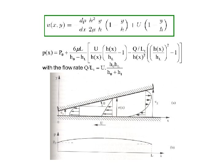
Other example of Laminar flow with Re>>1: Lubrication hypothesis (small inclination) cf. planar flow with x‐dependence Poiseuille + Couette

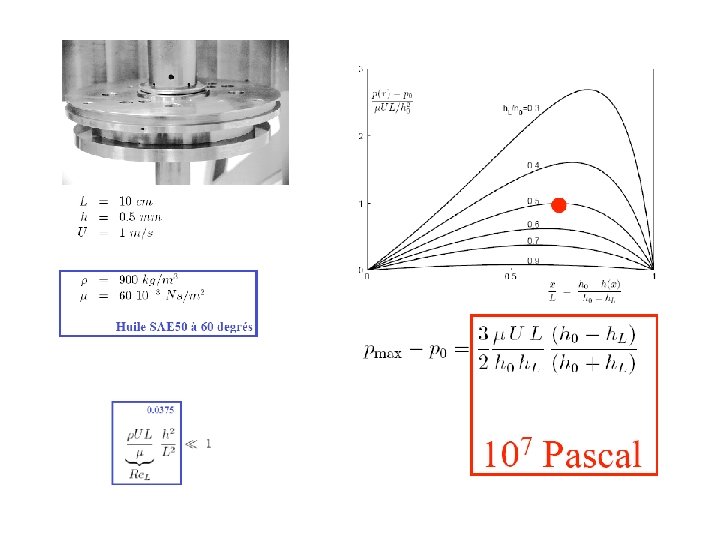
r=1. 2 kg. m‐ 3 h=2. 10‐ 5 Pa. s L ~ 1 m, h ~ 1 cm, U ~ 0. 1 m/s Re ~ 6000< (L/h)2 = 10000 x. M ~ e 1. L/h ~ 10 cm Supporting pressure PM ~ 10‐ 1 Pa

Flow above an obstacle: hydraulic swell Mass conservation: U. h=U(x). h(x) (I) Bernouilli along a streamline close to the surface: then (II) Case (I): d. U/dx(xm)=0 then U 2(x)‐gh(x)<0 then U(x) and h(x) Case (II): d. U/dx(x) >0 then U 2(xm)‐gh(xm)=0 then U(x) and h(x) U 2(x)‐gh(x) <0 becomes >0 low velocity of surfaces waves Hydraulic swell

End of Part I.