Markov Chain Monte Carlo MCMC The genie cannot

Markov Chain Monte Carlo (MCMC)

“The genie cannot be put back into the bottle. The Bayesian machine, together with MCMC, is arguably the most powerful mechanism ever created for processing data and knowledge” Berger (2000) “Gibbs sampling can be dangerous” BUGs project documentation

How to specify a Bayesian model • Write down the deterministic model of the ecological process • Write down the numerator of Bayes law in terms of the parameters in your deterministic model and the uncertainties. • Choose appropriate distributions for all probabilities. • Choose values for priors. • Done.

DH Rumsfeld on uncertainty “As we know, there are knowns. These are things we know that we know. There also known unknowns. That is to say, there are some things that we know we don’t know. But there also unknowns, the ones we don’t know”. DOD briefing Feb. 12, 2002

Exercise: write a Bayesian model for the model of light Limitation of Trees ϒ= max. growth rate at high light c=minimum light requirement α=slope of curve at low light

Bayesian Networks The heads of the arrows specify variables on the left hand side of the conditioning in the joint distribution; the tails are on the right hand Side. Anything without an arrow leading to it is either known as data or “known” as a prior with numeric arguments. If the prior is uninformative, these quantities are “known unknowns”. They are also called “directed acyclic graphs (DAG)” and “Bayesian belief networks”

Process model Parameter model

The integration cannot be done except for simple , conjugate models. What now?

What we are seeking: the posterior distribution P(θ|y) Note that we are dividing each point the dashed line by the area in the dashed line to obtain a probability reflecting our prior and current knowledge.

Breathe through your left nostril

Some intuition for what we are doing Because P(y) is a normalizing constant And when the prior is uninformative: So, estimating the posterior requires that we “normalize the likelihood” using numerical methods. In the case where the priors contain information, we must normalize the product of the likelihood and the prior.

A simple example • We are interested in estimating the prevalence (theta) of the chrytid fungus in a population of frogs. • We are sort of lazy, so we only sample 12 frogs of which 3 are infected. • What is our best estimate of prevalence? • You could calculate the posterior with one equation but that’s not the point. • By the way, how would you calculate the posterior?

Direct calculation of posterior

Some intuition for what we are doing: notice these are exactly the same shape Posterior : beta (alpha=4, beta=10) Prob(theta|y) Likelihood binom(k=3, n=12, prob=theta)

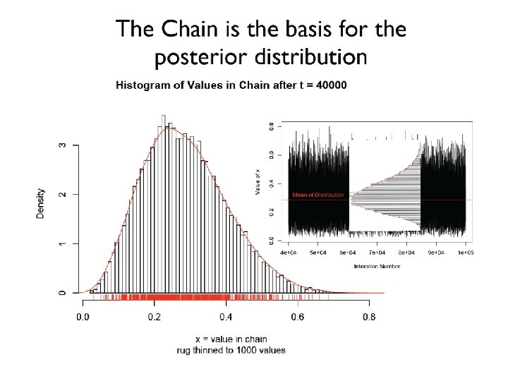
Some intuition for what we are doing: How do you normalize a histogram? The rug

What is our goal in MCMC? • The posterior distribution is unknown but the likelihood is known as are likelihood profiles. • We want to accumulate many, many values that represent random samples from the posterior distribution (the rug). • MCMC generates samples from unknown posterior distribution using the likelihood and the priors. In essence, it normalizes the likelihood multiplied by the prior in the same way we normalize a histogram. • We can then use these samples (the rug) to calculate statistics describing the distribution: means, medians, variances, etc. We can then use them to plot the posterior in the same way in which we normalize a histogram with lots and lots of data. • This is not magic, honest

But, how do you generate data from something that is unknown? It isn’t entirely unknown, really, because we know the likelihood (In this example the prior is uninformative) Posterior Prob(theta|y) Likelihood

Breathe through your left nostril

Intuition for MCMC: Creating the rug of values using Metropolis algorithm MCMC outputs the rug as an ordered vector θ=x, containing elements xt where t=1, ……n. xt=value of vector at time t Zt+1= proposed new value of vector at next step in chain We have a probability rule that allows us to compare the proposed new value z with the current value of x. If z is more probable than x, it becomes x. Otherwise, we keep x. This provides us with the rug of values for θ.

Remember the x’s are our estimates of θ The Rug t 1 Proposal (z) z 2 Rule Chain (x) 2 p(z 2)>p(x 1) x 1 x 2=z 2 3 4 z 3 z 4 p(x 2)>p(z 3) p(x 3)>p(z 4) x 3=x 2 x 4=x 3 5……………n z 5……………zn p(z 5)>p(x 4) x 5=z 5…. As the chain gets longer, the more probable values are retained more frequently than the less probable ones. This is what gives the proper shape to the simulated distribution.

The wickedly clever idea behind MCMC • We don’t know the posterior distribution of θ, but we can simulate its density using a series of random draws accumulated in a Markov chain. • The priors and the data, acting through the likelihoods, arbitrate which draws are kept in the chain and which are rejected.

Metropolis: The simplest MCMC We start with an arbitrary value of θ=x 1. We then draw a new value for θ, zt+1, from an arbitrary symmetric probability distribution (more about symmetry to follow). We calculate the ratio of the two, R.

The clever bit

Metropolis algorithm • Calculate R based on likelihoods and prior distributions (i. e. , the numerator of Bayes law). • Draw a random number U from a uniform distribution between 0 and 1. • If R > U, we keep zt+1 as the next value in the chain. Otherwise, we keep x 1 as the next value.

You will also see • Calculate R based on likelihoods and prior distributions (i. e. , the numerator of Bayes law). • Draw a random number U from a uniform distribution between 0 and 1. • If R≥ 1, we keep zt+1 as the next value in the chain. • If R≤ 1, we keep zt+1 as the next value in the chain with probability R and keep x 1 with probability 1 -R.

You will also see Keep z as the next value in the chain with probability R and keep x with probability (1 -R)

Breathe through your left nostril

A simple example • We are interested in estimating the prevalence (p) of the chrytid fungus in a population of frogs. • We are sort of lazy, so we only sample 12 frogs of which 3 are infected. • What is our best estimate of prevalence? • You could calculate the posterior with one equation but that’s not the point. • By the way, how would you calculate the posterior?

Derivation of beta-binomial conjugate prior We want to estimate the posterior distribution of the parameter p, the proportion of successes on n trials with y successes. Using Bayes theorem:

Direct calculation of posterior

The setup • Data= 3 successes (y) out of 12 trials (n) • Likelihood: binomial(s=3|θ, n=12) • We want to estimate P(θ|y), the posterior distribution of θ. • We assume that we have no prior information. • The numerator of Bayes theorem:

The pieces of Metropolis A function for the likelihood A function for the prior A vector to store the chain (retained values) An initial guess at the parameter value A vector containing random draws from a specified proposal distribution • A vector containing uniform 0 -1 random variables to make decisions whether to keep the current value in the chain or the proposed new value. • • •

Exercise: the fungus • Implement the algorithm for Metropolis sampler to estimate φ, the chrytid fungus prevalence. • Use a uniform 0 -1 as your proposal distribution. Assume no prior information, that is, prior(φ)=uniform(0, 1). [You could also use beta but this might convince you skeptics…] • Plot the known and estimated value of φ as a function of the number of iterations. • Plot the estimated posterior distribution of φ (smooth or a histogram) and overlay the exact calculation of the posterior.

ni = 200000 #number of steps in chain burnin=10000 x = numeric(ni) #vector to hold chain for phi x[1] = 0. 1 #initial value for chain z = runif(ni, 0, 1) # proposal distribution u = runif(ni, 0, 1) #decision vector # likelihood function L=function(phi)dbinom(3, size=12, prob=phi) #uninformative prior for phi =uniform prior between 0 and 1 pr=function(m)dunif(x=m, min=0, max=1) # move through the chain for(j in 2: ni){ #get ratio of likelihoods * priors ratio = L(z[j]) *pr(z[j]) / L(x[j-1])*pr(x[j-1]) #decide whether to keep proposal if (u[j] < ratio) x[j] = z[j] else x[j] = x[j-1] }

First 20 iterations from chain z (prop) 1 0. 1 2 0. 188121 3 0. 188121 4 0. 188121 5 0. 428743 6 0. 428743 7 0. 428743 8 0. 428743 9 0. 428743 U 0. 087806 0. 188121 0. 715242 0. 709325 0. 428743 0. 879641 0. 677814 0. 660766 0. 961057 R 0 2. 633613 0. 004415 0. 005182 0. 500428 7. 07 E-06 0. 022815 0. 033617 3. 58 E-10 10 0. 428743 11 0. 178869 12 0. 248837 13 0. 248837 14 0. 137459 15 0. 137459 16 0. 137459 17 0. 47695 18 0. 498773 19 0. 112981 20 0. 112981 0. 825173 0. 178869 0. 248837 0. 42574 0. 137459 0. 758926 0. 605179 0. 47695 0. 498773 0. 112981 0. 87345 0. 000168 1. 902138 1. 20791 0. 446744 0. 585039 0. 001752 0. 075286 0. 4632 0. 779313 1. 978771 1. 13 E-05 Yes No No No Yes No y … Calculate R based on likelihoods and prior distributions (i. e. , the numerator of Bayes law). [Proposed/Previous] Draw a random number U from a uniform distribution between 0 and 1. If R > U, we keep zt+1 as the next value in the chain. Otherwise, we keep x 1 as the next value. Prob (θ|data) j U<R accept? Question. Why doesn’t it get stuck at the MLE?

Prob (θ|data)

Prob (θ|data)

Prob (θ|data)

Prob (θ|data)

OK, that was nice. How about a real problem with multiple parameters? How do you use MCMC in that context?

Breathe through your left nostril

The essence of Gibbs sampling • We decompose a multivariate distribution into a series of univariate distributions called full conditional distributions. • We then cycle through each parameter for each iteration of the chain, sampling from the appropriate univariate distribution and treating the others as if they were known and constant.

Full conditional distributions Let θ be a vector of length k made of all the parameters we seek to estimate. Let θ-j be a vector of length k-1 including all elements of θ except θj. The full conditional distribution of θj is: P(θj |θ-j , y) It is the posterior distribution of θj conditioned on all the other parameters and the data.

The Gibbs sampler Presume we have a vector θ of three parameters. We will use the notation: to mean the posterior distribution of θ 1 assuming that θ 2 and θ 3 are known and constant. This is notation for the full conditional distribution that is a bit easier to see.

The Gibbs sampler We iterate over the chain sampling: At each step, we use the most recent values of the other parameters as “known and constant. ” So for example, in step 2, we use the value of θ 1 at time t and the value of θ 3 at time t-1.

The Gibbs sampler This generalizes to any number of parameters:

A Gibbs sampler with Gibbs steps for our draws from the posterior with each step in the chain • This is a critical concept. All Gibbs samplers require us to decompose the posterior into a series of univariate conditional distributions using simple rules. Each parameter that we wish to estimate has its own chain and we sample the parameters as if the others were known and constant at each step in the chain. The way we do that sampling is called a step. • Gibbs steps sample directly from the posterior distribution using conjugate prior relationships. • Metropolis and Metropolis-Hastings sample from the posterior by finding the most probable values from proposal distributions.

What’s ahead: sampling using: • • Metropolis steps Gibbs steps Metropolis-Hastings steps Hybrid steps. There are different acceptance rules for different algorithms. More on that later….

What’s ahead: Gibbs sampling using: • • Metropolis steps Gibbs steps Metropolis-Hastings steps Hybrid steps.

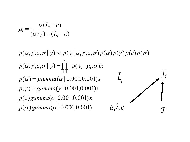
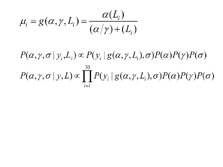
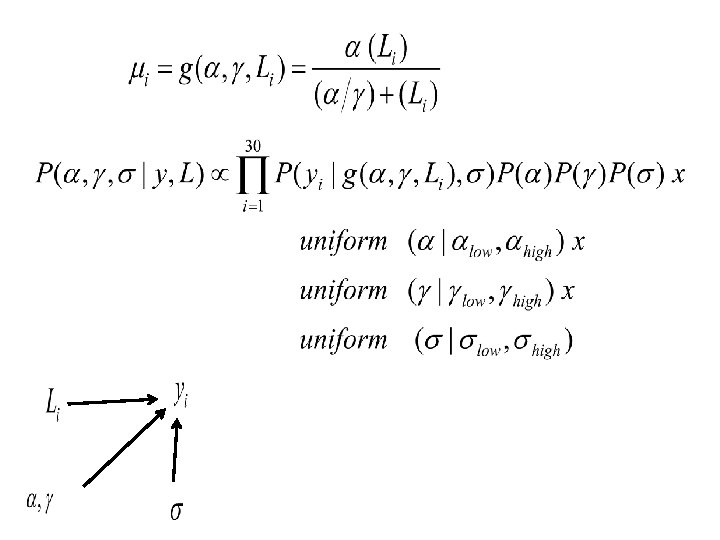
MCMC for a non-linear, multi-parameter model: Metropolis Steps: Back to the trees ϒ= max. growth rate at high light α=slope of curve at low light

Bayesian Networks The heads of the arrows specify variables on the left hand side of the conditioning in the joint distribution; the tails are on the right hand Side. Anything without an arrow leading to it is either known as data or “known” as a prior with numeric arguments. If the prior is uninformative, these quantities are “known unknowns”.

Now choose appropriate probability distributions for the likelihood and the priors. Remember, these cannot have > 3 arguments. All parameters must be positive.

Breathe through your left nostril

# Let's return to the hemlock trees looking for light # Generate some data with known parameter values. a=38. 5 b=1. 7 n = 50 sigma = 2 x=rgamma(50, shape=2, scale=20) # generate light values # Estimate deterministic growth true. growth=a*x/((a/b)+x) y=true. growth+rnorm(n, 0, sigma) plot(x, y) curve(a*x/((a/b)+x), add=T) # Fit model using nls() and get vector of coefficients model=nls(y~a*x/((a/b)+x), start=list(a=40, b=2)) summary(model) # Likelihood function L = function(a, b, sd, data = y){ pred = a*x/((a/b)+x) like = prod(dnorm(y, pred, sd)) return(like) }

# Define uninformative priors for the parameters prior. a = function(a) 1 prior. b = function(b) 1 prior. sigma=function(sigma) 1 # Number of simulations n. sim= 200000 burn. in=50000 # These are the simulations we will throw out # Set up data structures to hold simulaitons a = numeric(n. sim) b = numeric(n. sim) sigma = numeric(n. sim) # Define initial values for the parameters a[1] = 30; b[1] = 2 ; sigma[1] = 1 # Set up parameters for uniform proposal distributions a. low=20 a. up = 100 b. low = 1 b. up = 5 sigma. low = 0. 1 sigma. up = 5

# Create vectors of proposals prop. a = runif(n. sim, a. low, a. up) prop. b = runif(n. sim, b. low, b. up) prop. sigma = runif(n. sim, sigma. low, sigma. up) # these are used to test for keeping member of chain by comparing to ratio. u. a = runif(n. sim, 0, 1) u. b = runif(n. sim, 0, 1) u. sigma = runif(n. sim, 0, 1)

# The Gibbs Sampler for(j in 2: n. sim){ #update a ratio =L(a=prop. a[j], b=b[j-1], sd=sigma[j-1], data=y) * prior. a(prop. a[j]) / L(a=a[j-1], b=b[j-1], sd=sigma[j-1], data=y)* prior. a(a[j-1]) R = min(1, ratio) if(u. a[j] < R) a[j] = prop. a[j] else a[j] = a[j-1] #update b ratio = L(b=prop. b[j], a=a[j], sd=sigma[j-1]) * prior. b(prop. b[j]) / L(a=a[j-1], b=b[j-1], sd=sigma[j-1])* prior. b(b[j-1]) R = min(1, ratio) if(u. b[j] < R) b[j] = prop. b[j] else b[j] = b[j-1] # update sigma ratio = L(a=a[j], b=b[j], sd=prop. sigma[j]) * prior. sigma(prop. sigma[j]) / L(a=a[j-1], b=b[j-1], sd=sigma[j-1])* prior. sigma(sigma[j-1]) R = min(1, ratio) if(u. sigma[j] < R) sigma[j] = prop. sigma[j] else sigma[j] = sigma[j-1] }

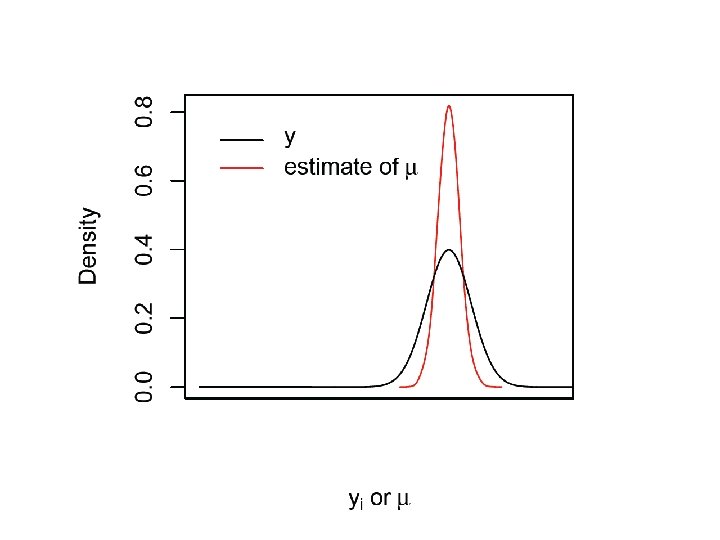
# Compare results from nls and mcmc print("nls summary") summary(model) mcmc. sum<-rbind(quantile(a[burn. in: n. sim], prob=c(0. 05, 0. 5, . 95)), quantile(b[burn. in: n. sim], prob=c(0. 05, 0. 5, . 95)), quantile(sigma[burn. in: n. sim], prob=c(0. 05, 0. 5, . 95))) rownames(mcmc. sum)<-c("a", "b", "sigma") mcmc. Sum # plot chains par(mfrow=c(2, 2)) plot(a, typ='l'); abline(h=mean(a[burn. in: n. sim]), col='red') plot(b, typ='l'); abline(h=mean(b[burn. in: n. sim]), col='red') plot(sigma, typ='l'); abline(h=mean(sigma[burn. in: n. sim]), col='red') # plot posterior distributions par(mfrow=c(2, 2)) plot(density(a[burn. in: n. sim], adjust=4), main="a"); abline(v=mean(a[burn. in: n. sim]), col='red') plot(density(b[burn. in: n. sim], adjust=4), main="b"); abline(v=mean(b[burn. in: n. sim]), col='red') plot(density(sigma[burn. in: n. sim], adjust=4), main="sigma") abline(v=mean(sigma[burn. in: n. sim]), col='red')

Gibbs steps • In the Gibbs step, we sample a parameter from the posterior distribution directly using conjugate -prior posterior relationships. • This is much more easily understood by example.

Recall that parameters themselves have distributions, right? The conjugate prior for the normal mean is normal, assuming variance is known. Shape parameters for the normal posterior are: Posterior μ Posterior σμ

The conjugate prior for the normal mean is normal, assuming variance is known. Shape parameters for the normal posterior are: σμprior = the prior estimate of the standard deviation of the distribution of the mean, μ σ2 = the standard deviation of the distribution that gives rise to the data. We must know the var Posterior μ Posterior σμ σμ = the posterior estimate of the standard deviation of the distribution of the mean, μ

Caution: When obtaining priors, you need to be careful about standard deviation and standard error. For a normal distribution, the standard deviation is the second shape parameter for the normal distribution of the random variable. The standard error is the second shape parameter for the normal distribution of the mean of the random variable (actual observations). The mean is the first shape parameter for both distributions.

The conjugate prior for a normal precision (τ=1/σ2), with known mean is gamma. Shape parameters for the gamma posterior are: We must know the mean

Example of Gibbs steps within a Gibbs sampler • We have 50 observations of the difference in biomass in plots from a grazed grassland in June and August. A normal distribution for the likelihood is a logical choice because the values are continuous and could be positive or negative. • We want to estimate the posterior distributions of the mean and standard deviation of the difference in biomass. We have prior information on the mean difference in biomass= 22. 7 g/m 2, standard deviation of the mean (i. e. , s. e. )=3. 8 g/m 2. We have no prior information on the standard deviation of the difference in biomass. • We can use the normal-normal conjugate prior to estimate the mean, but this assumes we know the variance. • We can use a gamma-gamma conjugate prior to estimate the precision, but this means we know the mean.

The model For a single data point:

We construct a Gibbs sampler We first write the conditional distributions for the parameters we want to estimate. These are univariate distributions containing each parameter. They are univariate because we treat other parameters as known and constant-there is only one parameter in the LHS of the equation.

We use a Gibbs sampler μ=new estimate of mean, σ=new standard deviation We iterate over t, sampling sequentially from: The full conditional distributions At each step, we use the most recent values of other parameters as “known and constant”.

Breathe through your left nostril

Algorithm • Set up some storage vectors for μ and σ. • Set initial conditions for μ and σ. • Make a draw of μ from its normal-normal conjugate posterior using the current value of σ. Store it in chain. • Make a draw of τ from its gamma-gamma conjugate posterior using the current value of μ. Store it in chain. • Calculate the current value of σ as 1/sqrt(τ). Store it in the σ chain. • Repeat until chain has converged.

# Generate some data n=50; y=rnorm(n, 30. 7, 4) mu. data<-mean(y) sd. data<-sqrt(sum((y-mu. data)^2)/n); var. data<-sd. prior^2 # Assume no prior information on distribution of mean or precision mu. prior=0; sd. prior=1000; var. prior=sd. prior^2 shape. prior=0. 0001; rate. prior=0. 0001 # or incorporate prior information…. mu<-function(mu. prior, var. prior, y, sigma){ # using what we know, sigma mean=(mu. prior/var. prior)+sum(y)/sigma^2/(1/var. prior+n/sigma^2) sd=(sqrt(1/var. prior+ n/sigma^2))^-1 return(list(mean=mean, sd=sd))} sigma=sd. data # check my function mu(mu. prior, var. prior=var. prior, y=y, sigma=sigma) mean(y) tau<-function(shape. prior, rate. prior, y, mu){ # using what we know, mu shape=shape. prior+n/2 rate=rate. prior+sum((y-mu)^2)/2 return(list(shape=shape, rate=rate))} m=tau(shape. prior=shape. prior, rate. prior=rate. prior, y=y, mu=mean(y)) 1/sqrt(m$shape/m$rate) sd. data

iter=500000 #storage for chains x. tau=numeric(iter) x. mu=numeric(iter) x. sigma=numeric(iter) # Initial values x. mu[1]=0 x. sigma[1]=3 for(t in 2: iter){ # draw from posterior for mean using mu and tau functions on previous slide mu. shape=mu(mu. prior=mu. prior, var. prior=var. prior, y=y, sigma=x. sigma[t-1]) x. mu[t]=rnorm(1, mu. shape$mean, mu. shape$sd) # draw from posterior for precision tau. shapes=tau(shape. prior=shape. prior, rate. prior=rate. prior, y=y, mu=x. mu[y]) x. tau[t]=rgamma(1, tau. shapes$shape, tau. shapes$rate) x. sigma[t]=1/sqrt(x. tau[t])} mean(x. mu); mean(y) mean(x. sigma); sd. data