The Monte Carlo method The Monte Carlo mehod



![Sampling by Inversion By construction: u(y) is the Uniform distribution in [0, 1] yielding: Sampling by Inversion By construction: u(y) is the Uniform distribution in [0, 1] yielding:](https://slidetodoc.com/presentation_image/b7962b9fc94ea1958fa56bd0e992abdf/image-23.jpg)
![Sampling by Accept/Reject Algorithm: 1. Draw rx in [a, b] 2. Draw ry in Sampling by Accept/Reject Algorithm: 1. Draw rx in [a, b] 2. Draw ry in](https://slidetodoc.com/presentation_image/b7962b9fc94ea1958fa56bd0e992abdf/image-25.jpg)
![Assignments 1. Integrate f(x) =x^{-1/3} + 0. 1*x within [0, 1] using i) your Assignments 1. Integrate f(x) =x^{-1/3} + 0. 1*x within [0, 1] using i) your](https://slidetodoc.com/presentation_image/b7962b9fc94ea1958fa56bd0e992abdf/image-30.jpg)

- Slides: 32

The Monte. Carlo method The Monte. Carlo mehod is a general and powerful method to compute hyper-dimensional integrals, as they often occur in statistical mechanics and MANY other areas of science. Official credit: N. Metropolis, M. Rosenbluth, A. Teller, E. Teller, (1953), but it may go back to Fermi… Most valuable for systems at EQUILBRIUM, although dynamic versions exist as well (Kinetic Monte Carlo) Sauro Succi 1

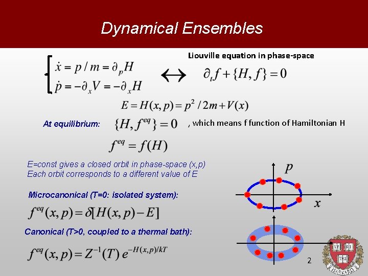
Dynamical Ensembles Liouville equation in phase-space At equilibrium: , which means f function of Hamiltonian H E=const gives a closed orbit in phase-space (x, p) Each orbit corresponds to a different value of E Microcanonical (T=0: isolated system): Canonical (T>0, coupled to a thermal bath): 2

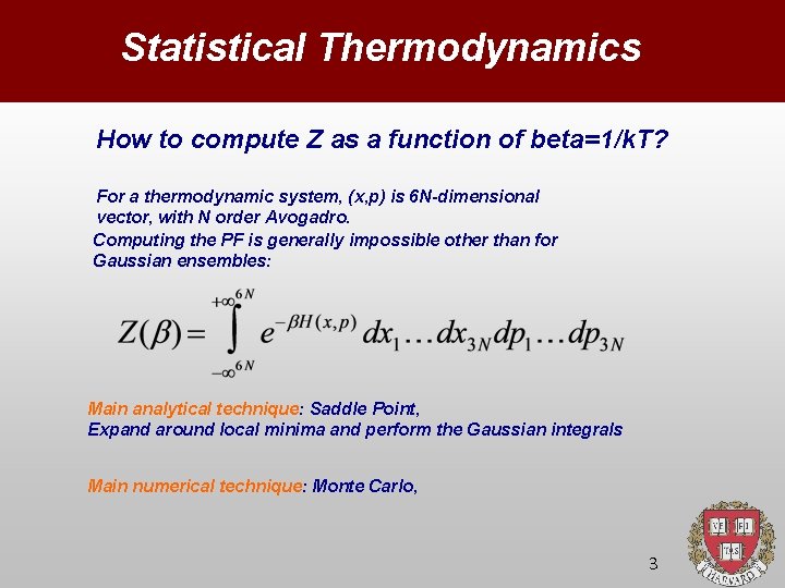
Statistical Thermodynamics How to compute Z as a function of beta=1/k. T? For a thermodynamic system, (x, p) is 6 N-dimensional vector, with N order Avogadro. Computing the PF is generally impossible other than for Gaussian ensembles: Main analytical technique: Saddle Point, Expand around local minima and perform the Gaussian integrals Main numerical technique: Monte Carlo, 3

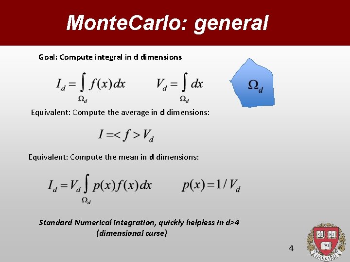
Monte. Carlo: general Goal: Compute integral in d dimensions Equivalent: Compute the average in d dimensions: Equivalent: Compute the mean in d dimensions: Standard Numerical Integration, quickly helpless in d>4 (dimensional curse) 4

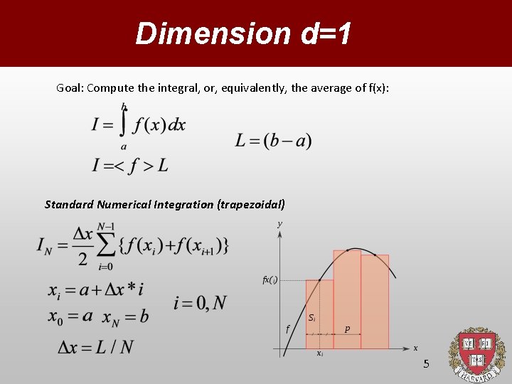
Dimension d=1 Goal: Compute the integral, or, equivalently, the average of f(x): Standard Numerical Integration (trapezoidal) 5

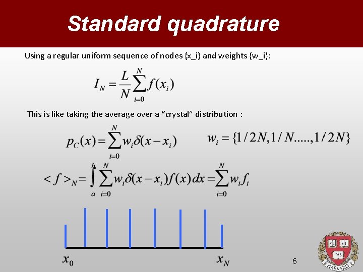
Standard quadrature Using a regular uniform sequence of nodes {x_i} and weights {w_i}: This is like taking the average over a “crystal” distribution : 6

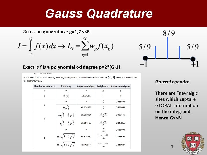
Gauss Quadrature Gaussian quadrature: g=1, G<<N Exact is f is a polynomial od degree p=2*(G-1) Gauss-Legendre There are “nevralgic” sites which capture GLOBAL information on the integrand. Hence G<<N 7

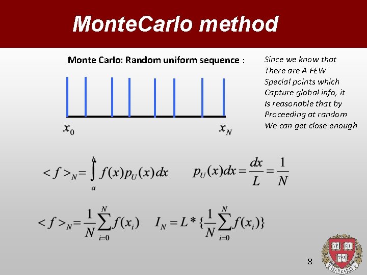
Monte. Carlo method Monte Carlo: Random uniform sequence : Since we know that There are A FEW Special points which Capture global info, it Is reasonable that by Proceeding at random We can get close enough 8

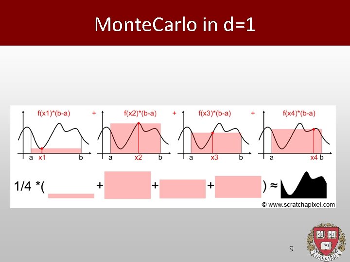
Monte. Carlo in d=1 9

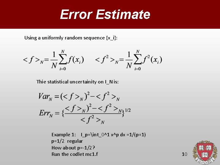
Error Estimate Using a uniformly random sequence {x_i}: Thie statistical uncertainity on I_N is: Example 1: I_p=int_0^1 x^p dx =1/(p+1) p=1/2 regular How about p=-1/2? Run the codlet mc 1. f 10

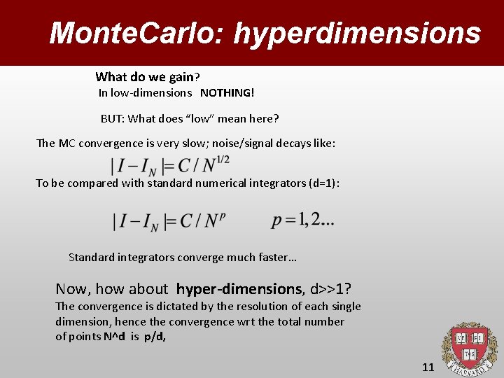
Monte. Carlo: hyperdimensions What do we gain? In low-dimensions NOTHING! BUT: What does “low” mean here? The MC convergence is very slow; noise/signal decays like: To be compared with standard numerical integrators (d=1): Standard integrators converge much faster… Now, how about hyper-dimensions, d>>1? The convergence is dictated by the resolution of each single dimension, hence the convergence wrt the total number of points N^d is p/d, 11

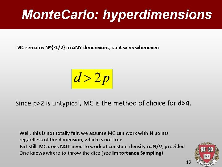
Monte. Carlo: hyperdimensions MC remains N^{-1/2} in ANY dimensions, so it wins whenever: Since p>2 is untypical, MC is the method of choice for d>4. Well, this is not totally fair, we assume MC can work with N points regardless of the dimension, which is not true. But still, MC does NOT need to work at constant density n=N/V, provided One knows where to throw the dice (see Importance Sampling) 12

MC strategy Grid methods cover the entire space uniformly. including regions where the function is vain, whence its inefficiency in d>>1. Gaussian quadrature is much smarter, but still inane at very large dimensions since for large d, G^d is unsustainable even with very small G. For instance G=3, d=20, 3^20 =3. 5 billions… So for d in the order of tens or more, MC is again the winner. Since MD is “blind” its efficiency is ver sensitive to localization: Ideal function: f(x)=Const. Just ONE shot is sufficient, since ANY x returns the correct answer: I=Const*Volume !!! Often, however, the volume itself is unknown! 13

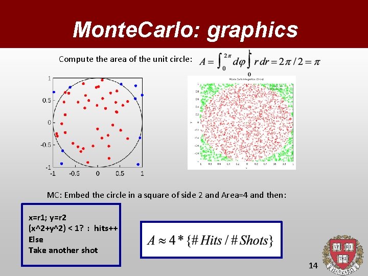
Monte. Carlo: graphics Compute the area of the unit circle: MC: Embed the circle in a square of side 2 and Area=4 and then: x=r 1; y=r 2 (x^2+y^2) < 1? : hits++ Else Take another shot 14

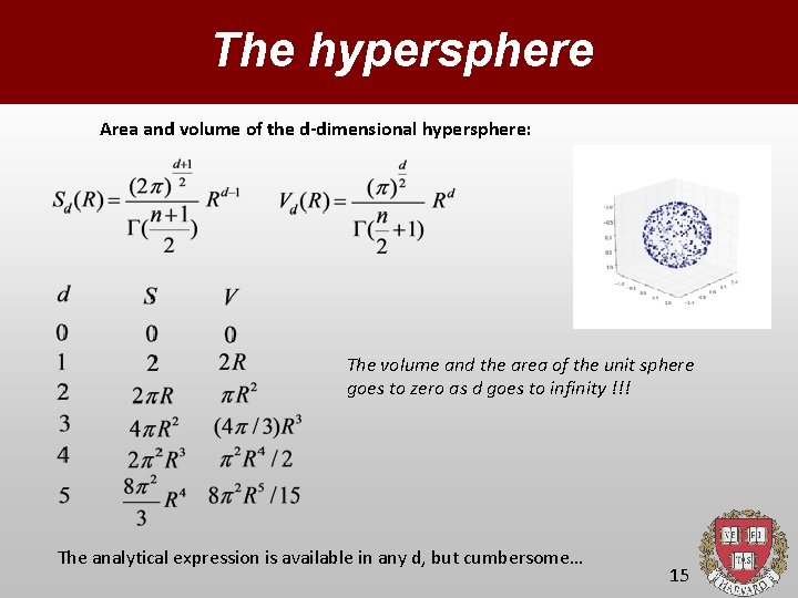
The hypersphere Area and volume of the d-dimensional hypersphere: The volume and the area of the unit sphere goes to zero as d goes to infinity !!! The analytical expression is available in any d, but cumbersome… 15

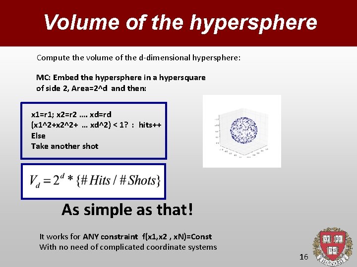
Volume of the hypersphere Compute the volume of the d-dimensional hypersphere: MC: Embed the hypersphere in a hypersquare of side 2, Area=2^d and then: x 1=r 1; x 2=r 2 …. xd=rd (x 1^2+x 2^2+ … xd^2) < 1? : hits++ Else Take another shot As simple as that! It works for ANY constraint f(x 1, x 2 , x. N)=Const With no need of complicated coordinate systems 16

Sneaky shapes Compute the area of the are of the Nile river… Clearly the chance of hitting The Nile is epsilon on this Scale: very inefficient! Remedy: Adaptive Monte Carlo. Restrict the procedure to a sequence of locally refined boxes around the Nile 17

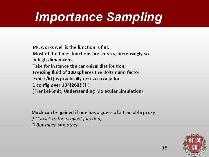
Importance Sampling MC works well is the function is flat. Most of the times functions are sneaky, increasingly so in high dimensions. Take for instance the canonical distribution: Freezing fluid of 100 spheres the Boltzmann factor exp(-E/k. T) is practically non-zero only for 1 config over 10^{260}!!!!! (Frenkel-Smit, Understanding Molecular Simulation) Much can be gained if one has a guess of a tractable proxy: i) “Close” to the original function, ii) But much smoother 18

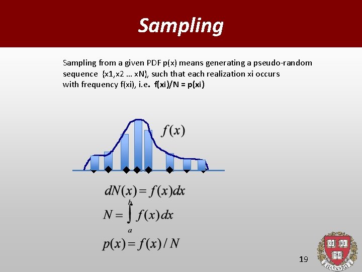
Sampling from a given PDF p(x) means generating a pseudo-random sequence {x 1, x 2 … x. N}, such that each realization xi occurs with frequency f(xi), i. e. f(xi)/N = p(xi) 19

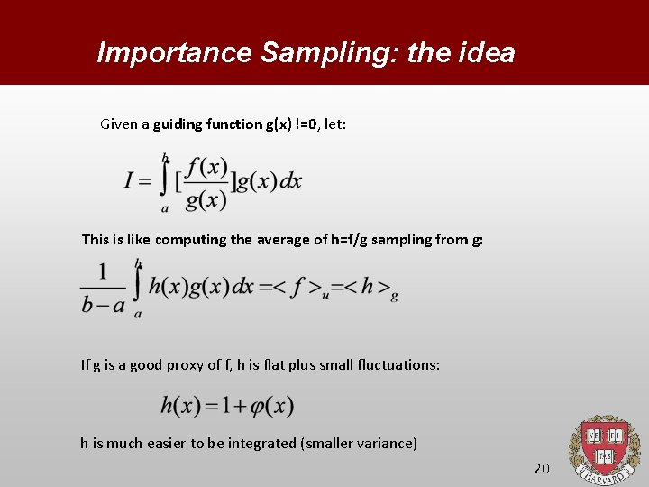
Importance Sampling: the idea Given a guiding function g(x) !=0, let: This is like computing the average of h=f/g sampling from g: If g is a good proxy of f, h is flat plus small fluctuations: h is much easier to be integrated (smaller variance) 20

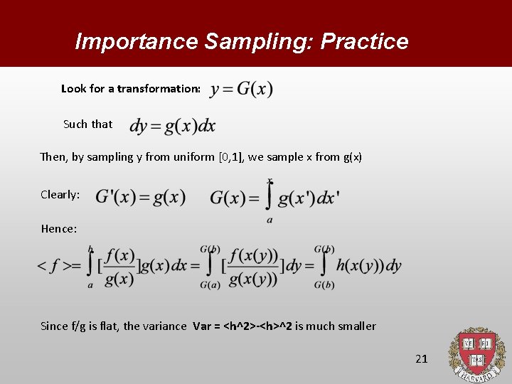
Importance Sampling: Practice Look for a transformation: Such that Then, by sampling y from uniform [0, 1], we sample x from g(x) Clearly: Hence: Since f/g is flat, the variance Var = <h^2>-<h>^2 is much smaller 21

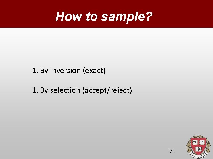
How to sample? 1. By inversion (exact) 1. By selection (accept/reject) 22
![Sampling by Inversion By construction uy is the Uniform distribution in 0 1 yielding Sampling by Inversion By construction: u(y) is the Uniform distribution in [0, 1] yielding:](https://slidetodoc.com/presentation_image/b7962b9fc94ea1958fa56bd0e992abdf/image-23.jpg)
Sampling by Inversion By construction: u(y) is the Uniform distribution in [0, 1] yielding: namely: Most x’s lie in the region of maximum slope of the CDF P(x): dx=dy/P’(x) This is optimal (efficiency =1) but requires explicit knowledge of the inverse CDF, which is most often unavailable especially in d>1. 23

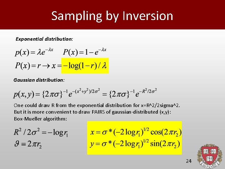
Sampling by Inversion Exponential distribution: Gaussian distribution: One could draw R from the exponential distribution for x=R^2/2 sigma^2. But it is more convenient to draw PAIRS of gaussian-distributed (x, y): Box-Mueller algorithm: 24
![Sampling by AcceptReject Algorithm 1 Draw rx in a b 2 Draw ry in Sampling by Accept/Reject Algorithm: 1. Draw rx in [a, b] 2. Draw ry in](https://slidetodoc.com/presentation_image/b7962b9fc94ea1958fa56bd0e992abdf/image-25.jpg)
Sampling by Accept/Reject Algorithm: 1. Draw rx in [a, b] 2. Draw ry in [f(a), f(b)] 3. Compute y=f(rx) 4. If y<ry: accept x=rx Else: Take another shot PROS: Very general, it applies to ANY dimensions! CONS: Low acceptance ratio for “sneaky” functions MC efficiency is considered OK for acceptance ratio > 50% 25

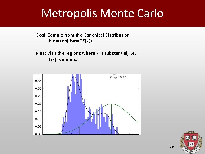
Metropolis Monte Carlo Goal: Sample from the Canonical Distribution P(x)=exp(-beta*E(x)) Idea: Visit the regions where P is substantial, i. e. E(x) is minimal 26

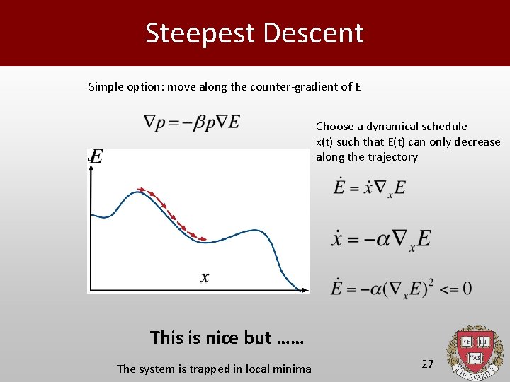
Steepest Descent Simple option: move along the counter-gradient of E Choose a dynamical schedule x(t) such that E(t) can only decrease along the trajectory This is nice but …… The system is trapped in local minima 27

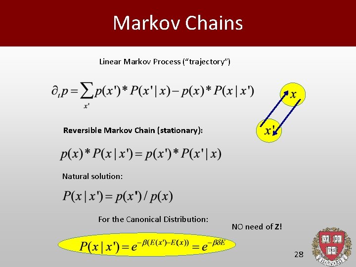
Markov Chains Linear Markov Process (“trajectory”) Reversible Markov Chain (stationary): Natural solution: For the Canonical Distribution: NO need of Z! 28

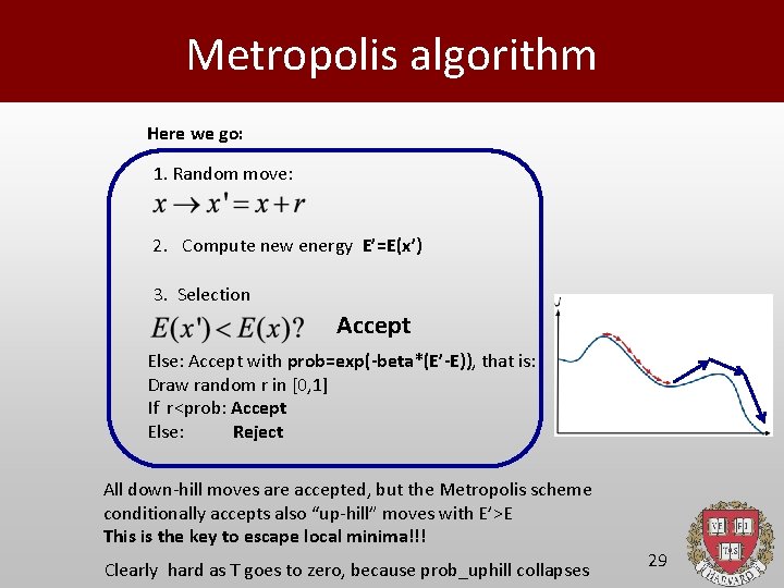
Metropolis algorithm Here we go: 1. Random move: 2. Compute new energy E’=E(x’) 3. Selection Accept Else: Accept with prob=exp(-beta*(E’-E)), that is: Draw random r in [0, 1] If r<prob: Accept Else: Reject All down-hill moves are accepted, but the Metropolis scheme conditionally accepts also “up-hill” moves with E’>E This is the key to escape local minima!!! Clearly hard as T goes to zero, because prob_uphill collapses 29
![Assignments 1 Integrate fx x13 0 1x within 0 1 using i your Assignments 1. Integrate f(x) =x^{-1/3} + 0. 1*x within [0, 1] using i) your](https://slidetodoc.com/presentation_image/b7962b9fc94ea1958fa56bd0e992abdf/image-30.jpg)
Assignments 1. Integrate f(x) =x^{-1/3} + 0. 1*x within [0, 1] using i) your quadrature of choice (Trapezoidal, Sympson. . . ) ii) Standard Monte Carlo iii) MC with importance sampling (see codlet mcis. f) 2. Compute the volume of the sphere in dimension d=1, 2, 3, 4, 5 using your best MC method. Plot the statistical error as a function of the number of samples. Does it scale like 1/sqrt(N)? 30

End of the lecture 31

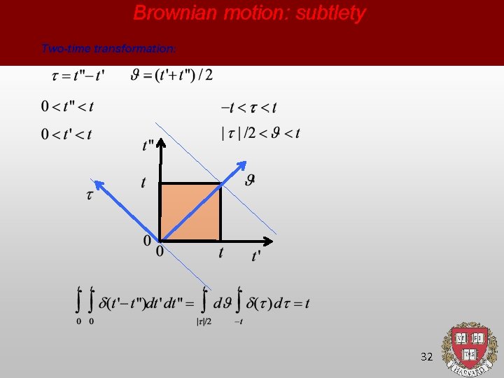
Brownian motion: subtlety Two-time transformation: 32