Junichi Yokoyama RESCEU The University of Tokyo M

Jun’ichi Yokoyama (RESCEU, The University of Tokyo) M. Kawasaki, T. Takayama, M. Yamaguchi & JY Physical Review D 74 (2006) 043525

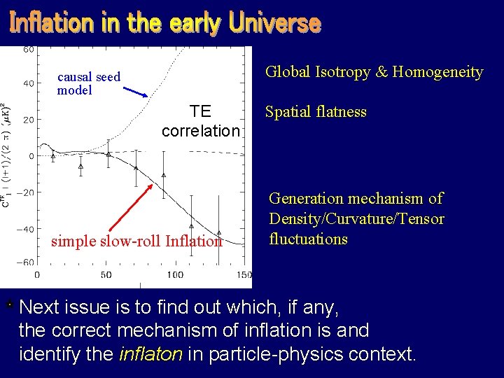
Global Isotropy & Homogeneity causal seed model T=2. 725 K Cosmic Microwave Background TE CMB Spatial flatness correlation simple slow-roll Inflation Generation mechanism of Density/Curvature/Tensor fluctuations Next issue is to find out which, if any, the correct mechanism of inflation is and identify the inflaton in particle-physics context.

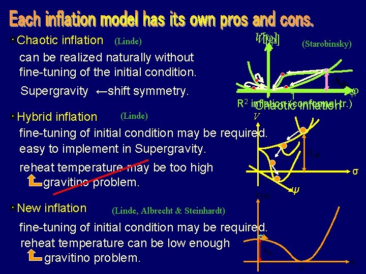
Chaotic inflation (Linde) can be realized naturally without fine-tuning of the initial condition. Supergravity ←shift symmetry. V[φ] V[σ] (Starobinsky) φ φ １ R 2 inflation (conformal １ inflationtr. )σ Chaotic V (Linde) Hybrid inflation fine-tuning of initial condition may be required. easy to implement in Supergravity. reheat temperature may be too high gravitino problem. New inflation (Linde, Albrecht & Steinhardt) fine-tuning of initial condition may be required. reheat temperature can be low enough gravitino problem. σ Ψ

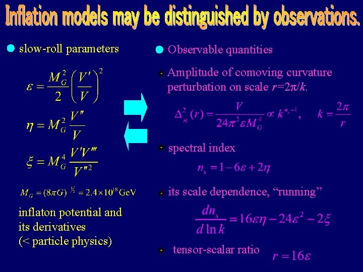
slow-roll parameters Observable quantities Amplitude of comoving curvature perturbation on scale r=2π/k. spectral index its scale dependence, “running” inflaton potential and its derivatives (< particle physics) tensor-scalar ratio

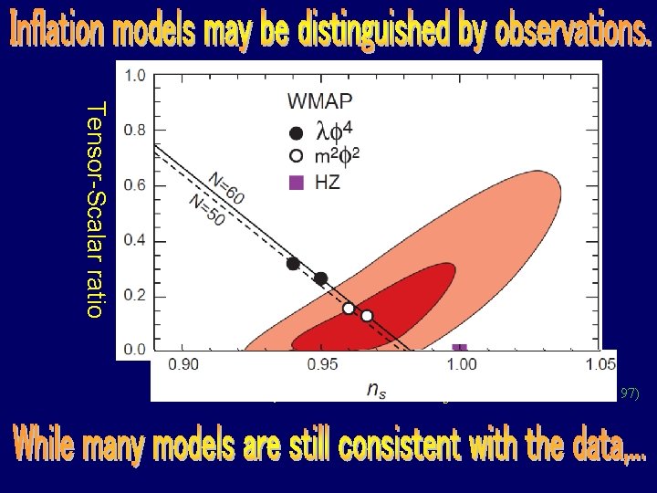
Tensor-Scalar ratio r. T 1 Chaotic Inflation 0. 5 Hybrid Inflation New Inflation 0 0. 8 0. 9 1 Spectral index ns 1. 1 (Dodelson, Kinney, Kolb 97)

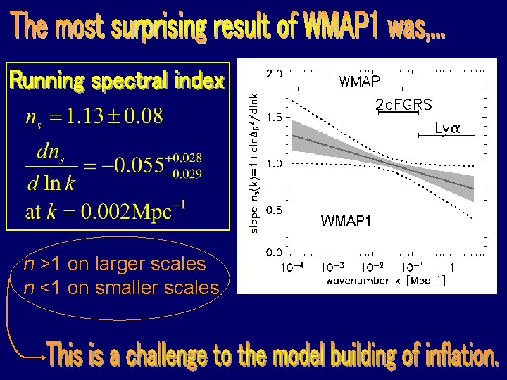
WMAP 1 n >1 on larger scales n <1 on smaller scales

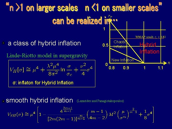
r. T 1 a class of hybrid inflation 0. 5 Linde-Riotto model in supergravity 0 Chaotic Inflation New Inflation 0. 8 0. 9 σ: inflaton for Hybrid Inflation smooth hybrid inflation Hybrid Inflation (Lazarides and Panagiotakopoulos) n 1 1. 1

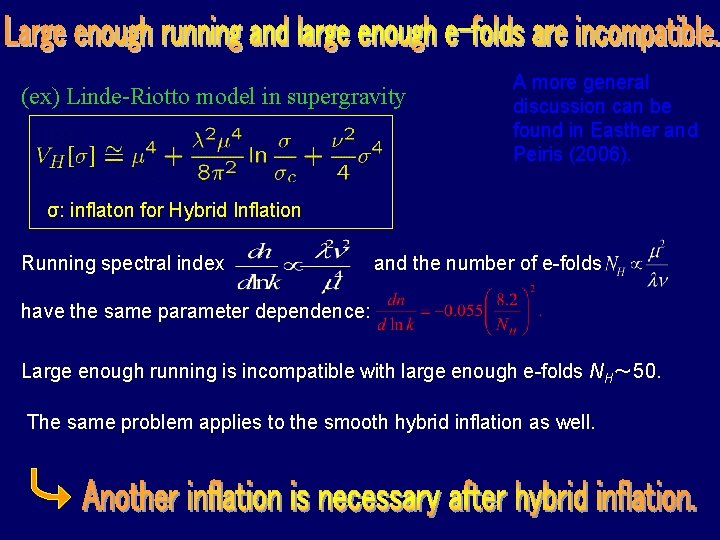
(ex) Linde-Riotto model in supergravity A more general discussion can be found in Easther and Peiris (2006). σ: inflaton for Hybrid Inflation Running spectral index and the number of e-folds have the same parameter dependence: Large enough running is incompatible with large enough e-folds NH～ 50. The same problem applies to the smooth hybrid inflation as well.

Inflation with a running spectral index in supergravity. M. Kawasaki, Masahide Yamaguchi, Jun'ichi Yokoyama Phys. Rev. D 68: 023508, 2003 Chaotic hybrid new inflation in supergravity with a running spectral index. Masahide Yamaguchi, Jun'ichi Yokoyama more natural initial condition Phys. Rev. D 68: 123520, 2003 Smooth hybrid inflation in supergravity with a running spectral index and early star formation. natural initial condition Masahide Yamaguchi, Jun'ichi Yokoyama no cosmic strings Phys. Rev. D 70: 023513, 2004 no one-loop correction

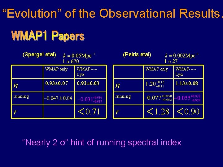
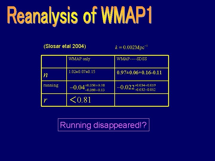
“Evolution” of the Observational Results… 　　　(Spergel etal) n 　　　(Peiris etal) WMAP only WMAP----Lyα 0. 93± 0. 07 0. 93± 0. 03 running r WMAP only n WMAP----Lyα 1. 13± 0. 08 running ＜ 0. 71 r ＜ 1. 28 ＜ 0. 90 “Nearly 2 σ” hint of running spectral index

(Slosar etal 2004) n WMAP only WMAP-----SDSS 1. 02± 0. 07± 0. 15 0. 97± 0. 06+0. 16 -0. 11 running r ＜ 0. 81 Running disappeared!?

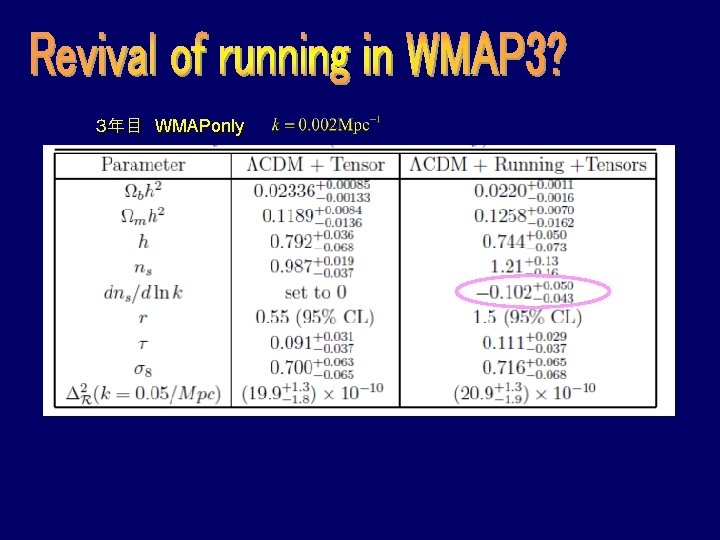
３年目　WMAPonly

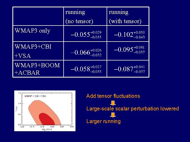
running (no tensor) running (with tensor) WMAP 3 only WMAP 3+CBI +VSA WMAP 3+BOOM +ACBAR Add tensor fluctuations Large-scale scalar perturbation lowered Larger running

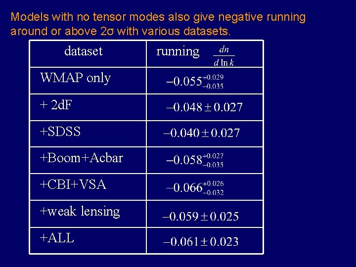
Models with no tensor modes also give negative running around or above 2σ with various datasets. dataset WMAP only + 2 d. F +SDSS +Boom+Acbar +CBI+VSA +weak lensing +ALL running

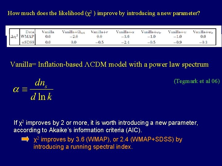
How much does the likelihood (χ2 ) improve by introducing a new parameter? Vanilla= Inflation-based ΛCDM model with a power law spectrum (Tegmark et al 06) If χ2 improves by 2 or more, it is worth introducing a new parameter, according to Akaike’s information criteria (AIC). χ2 improves by 3. 6 (WMAP), or 2. 4 (WMAP+SDSS) by introducing a running spectral index.

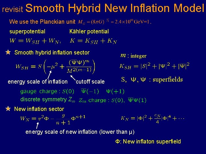
revisit Smooth Hybrid New Inflation Model We use the Planckian unit superpotential . Kähler potential Smooth hybrid inflation sector energy scale of inflation cutoff scale : integer S, : superfields discrete symmetry Zm New inflation sector energy scale of new inflation (lower than μ) Φ: New inflaton superfield

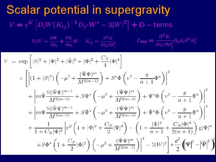
Scalar potential in supergravity

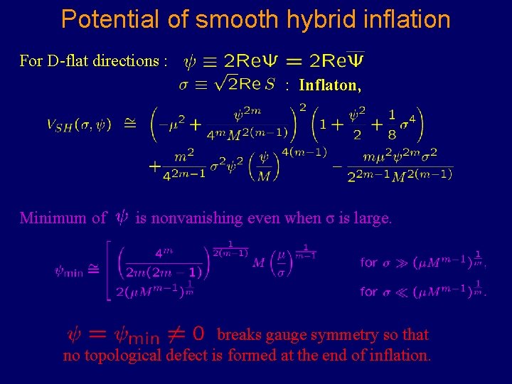
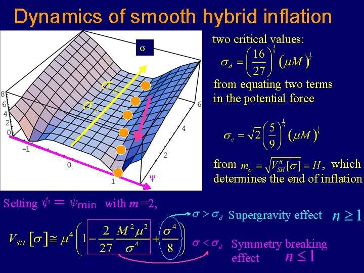
Potential of smooth hybrid inflation For D-flat directions : : Inflaton, Minimum of is nonvanishing even when σ is large. breaks gauge symmetry so that no topological defect is formed at the end of inflation.

Dynamics of smooth hybrid inflation two critical values: σ from equating two terms in the potential force ψ Setting with m =2, from , which determines the end of inflation Supergravity effect Symmetry breaking effect

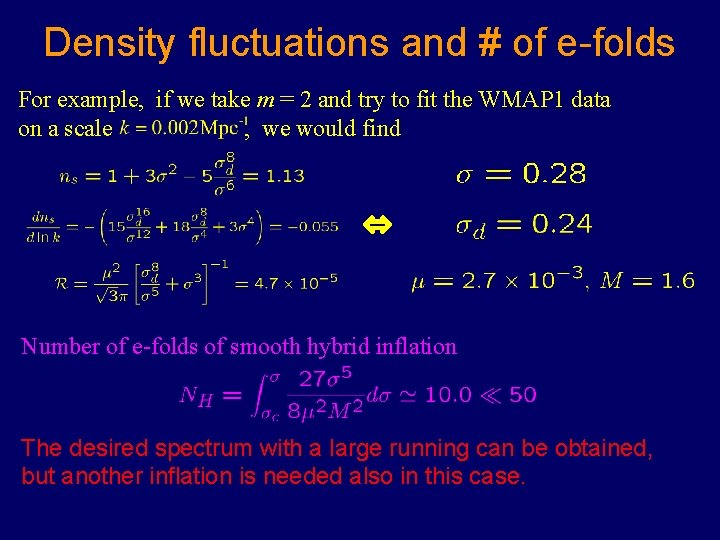
Density fluctuations and # of e-folds For example, if we take m = 2 and try to fit the WMAP 1 data on a scale , we would find ⇔ Number of e-folds of smooth hybrid inflation The desired spectrum with a large running can be obtained, but another inflation is needed also in this case.

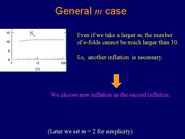
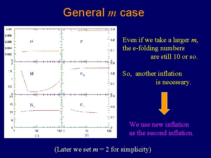
General m case Even if we take a larger m, the number of e-folds cannot be much larger than 10. So, another inflation is necessary. We choose new inflation as the second inflation. (Later we set m = 2 for simplicity)

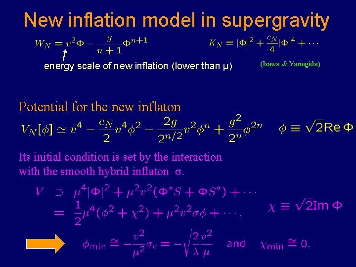
New inflation model in supergravity energy scale of new inflation (lower than μ) Potential for the new inflaton Its initial condition is set by the interaction with the smooth hybrid inflaton σ. (Izawa & Yanagida)

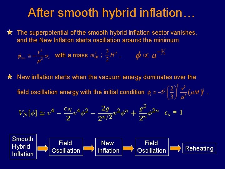
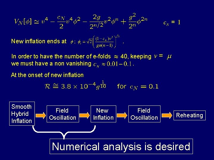
After smooth hybrid inflation… The superpotential of the smooth hybrid inflation sector vanishes, and the New Inflaton starts oscillation around the minimum with a mass . New inflation starts when the vacuum energy dominates over the field oscillation energy with the initial condition Smooth Hybrid Inflation Field Oscillation New Inflation Field Oscillation . Reheating

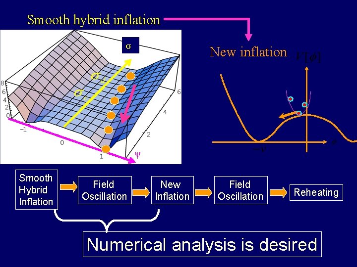
Smooth hybrid inflation σ New inflation ψ Smooth Hybrid Inflation Field Oscillation New Inflation Field Oscillation Reheating Numerical analysis is desired

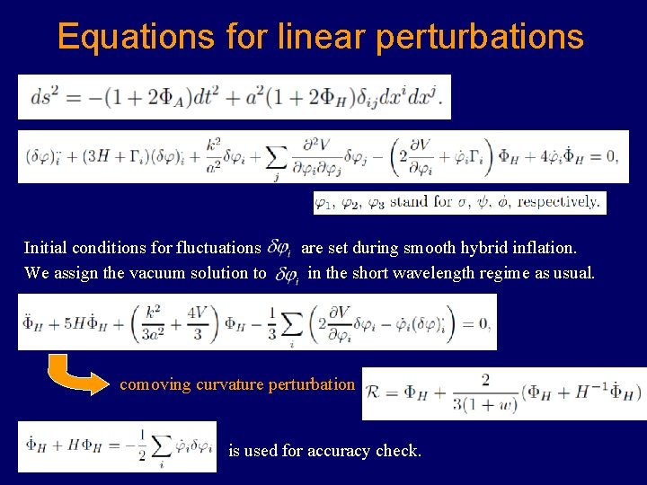
Equations for linear perturbations Initial conditions for fluctuations We assign the vacuum solution to are set during smooth hybrid inflation. in the short wavelength regime as usual. comoving curvature perturbation is used for accuracy check.

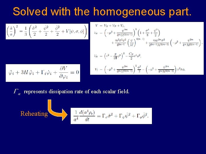
Solved with the homogeneous part. represents dissipation rate of each scalar field. Reheating

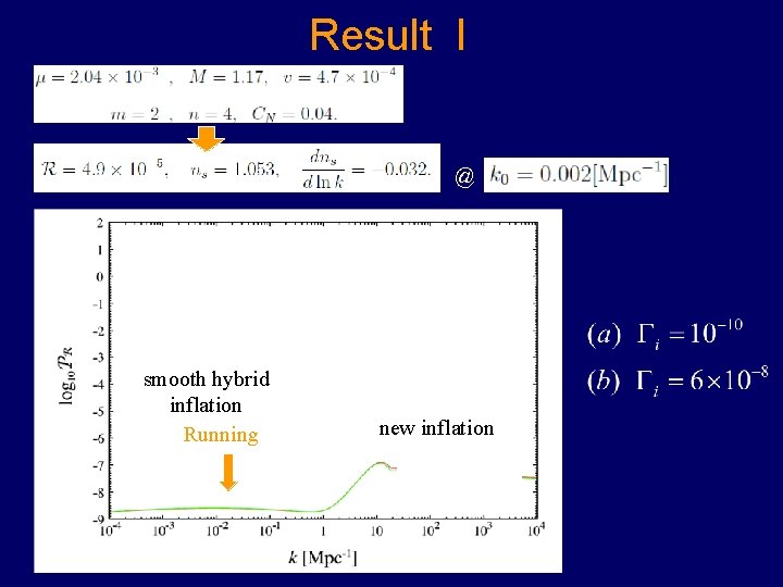
Result I @ smooth hybrid inflation Running new inflation

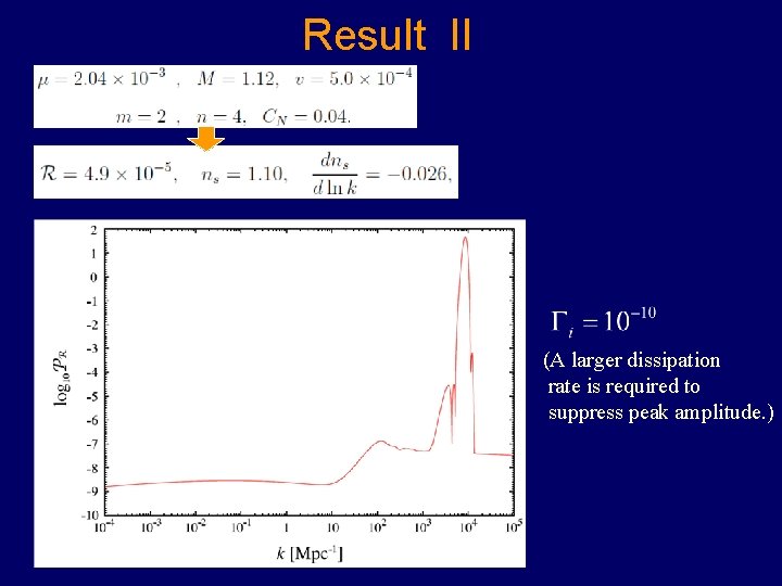
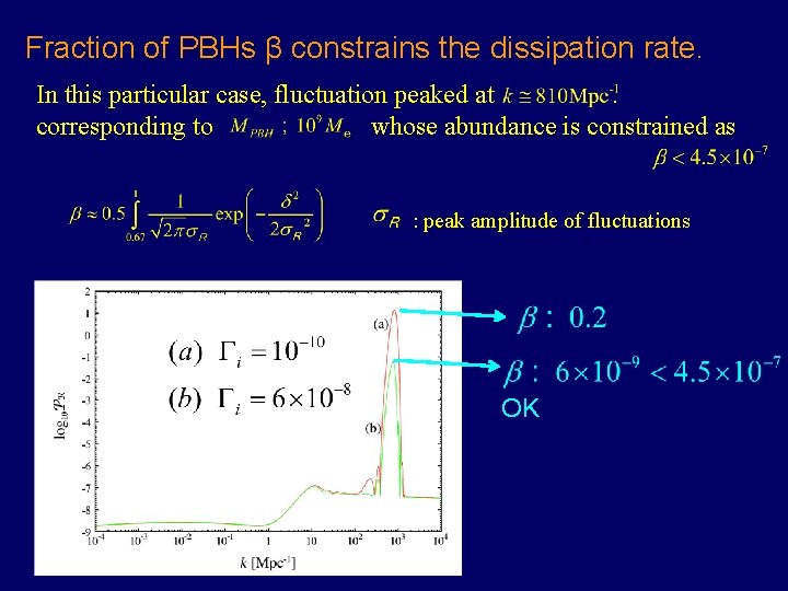
Result II (A larger dissipation rate is required to suppress peak amplitude. )

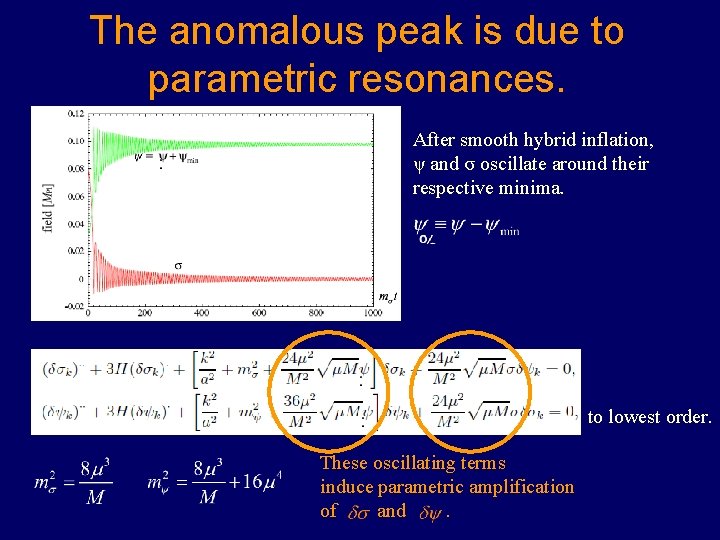
The anomalous peak is due to parametric resonances. After smooth hybrid inflation, ψ and σ oscillate around their respective minima. to lowest order. These oscillating terms induce parametric amplification of and.

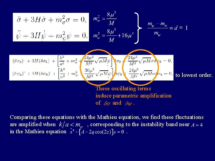
to lowest order. These oscillating terms induce parametric amplification of and. Comparing these equations with the Mathieu equation, we find these fluctuations are amplified when , corresponding to the instability band near in the Mathieu equation.

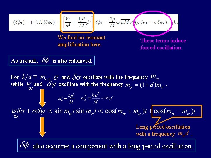
We find no resonant amplification here. As a result, For while is also enhanced. , and These terms induce forced oscillation. and oscillate with the frequency . Long period oscillation with a frequency. also acquires a component with a long period oscillation.

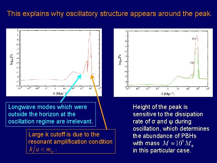
This explains why oscillatory structure appears around the peak. Longwave modes which were outside the horizon at the oscillation regime are irrelevant. Large k cutoff is due to the resonant amplification condition. Height of the peak is sensitive to the dissipation rate of σ and ψ during oscillation, which determines the abundance of PBHs with mass in this particular case.

Fraction of PBHs β constrains the dissipation rate. In this particular case, fluctuation peaked at. corresponding to whose abundance is constrained as : peak amplitude of fluctuations OK

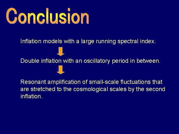
Inflation models with a large running spectral index. Double inflation with an oscillatory period in between. Resonant amplification of small-scale fluctuations that are stretched to the cosmological scales by the second inflation.

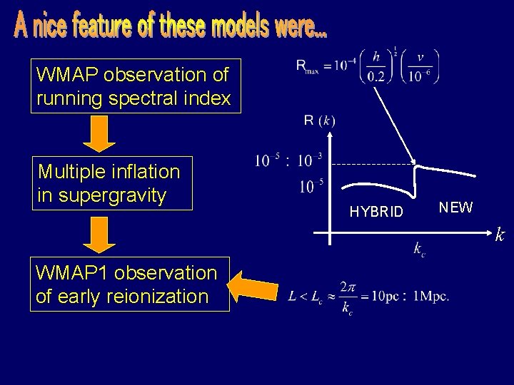
WMAP observation of running spectral index Multiple inflation in supergravity HYBRID NEW k WMAP 1 observation of early reionization

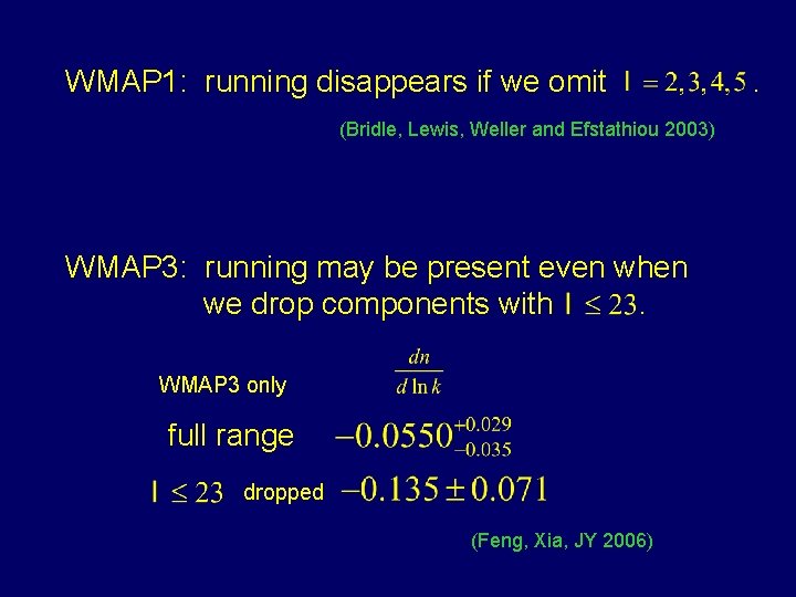
WMAP 1: running disappears if we omit (Bridle, Lewis, Weller and Efstathiou 2003) WMAP 3: running may be present even when we drop components with. WMAP 3 only full range dropped (Feng, Xia, JY 2006) .

General m case Even if we take a larger m, the e-folding numbers are still 10 or so. So, another inflation is necessary. We use new inflation as the second inflation. (Later we set m = 2 for simplicity)

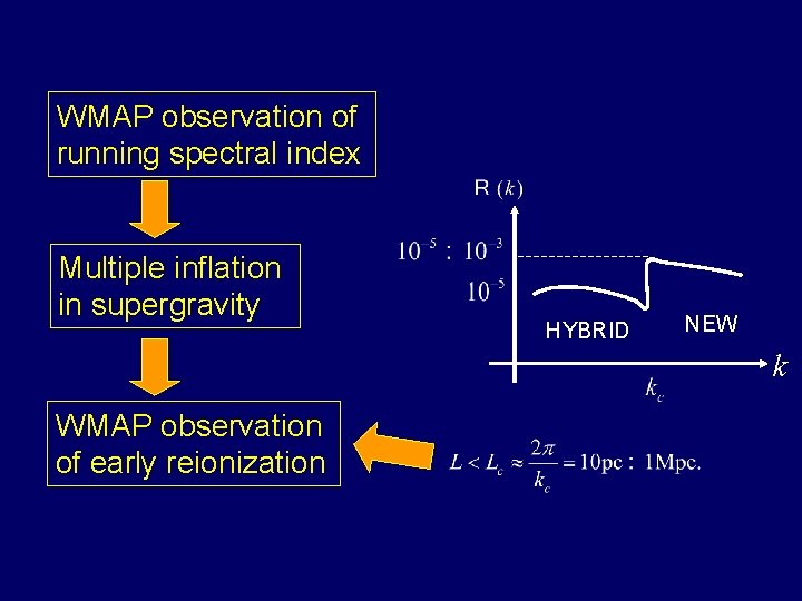
WMAP observation of running spectral index Multiple inflation in supergravity HYBRID NEW k WMAP observation of early reionization

New inflation ends at . In order to have the number of e-folds we must have a non vanishing 40, keeping. At the onset of new inflation Smooth Hybrid Inflation Field Oscillation New Inflation Field Oscillation Reheating Numerical analysis is desired