Infinite Impulse Response IIR Filters Learning Objectives u
 Filters")
Infinite Impulse Response (IIR) Filters

Learning Objectives u Introduction to theory behind IIR filters: w w w u Properties. Coefficient calculation. Structure selection. Implementation in Matlab, C and assembly.
 filters are the first choice when: w w")
Introduction u Infinite Impulse Response (IIR) filters are the first choice when: w w u u Speed is paramount. Phase non-linearity is acceptable. IIR filters are computationally more efficient than FIR filters as they require fewer coefficients due to the fact that they use feedback or poles. However feedback can result in the filter becoming unstable if the coefficients deviate from their true values.

Properties of an IIR Filter u The general equation of an IIR filter can be expressed as follows: u ak and bk are the filter coefficients.

Properties of an IIR Filter u The transfer function can be factorized to give: u Where: z 1, z 2, …, z. N are the zeros, p 1, p 2, …, p. N are the poles. u The filter is stable iff its poles reside inside the unit circle

Properties of an IIR Filter u The transfer function can be factorized to give: u For the implementation of the above equation we need the difference equation:

Properties of an IIR Filter IIR Equation IIR structure for N = M = 2

IIR Filters on a Computer u Filters may be implemented on a computer in 3 possible ways w w w u Using convolution Using the difference equation Using the frequency response For IIR filters only the implementation with the difference equation is possible: w w The impulse response is infinite, and direct convolution cannot be calculated Discrete Fourier Transform exists only for finite signals

Design Procedure u To fully design and implement a filter five steps are required: (1) (2) (3) (4) (5) Filter specification. Coefficient calculation. Structure selection. Simulation (optional). Implementation.

Filter Specification - Step 1

Coefficient Calculation - Step 2 u There are two different methods available for calculating the coefficients: w w u Direct placement of poles and zeros. Using analogue filter design. Both of these methods are described.

Placement Method u All that is required for this method is the knowledge that: w w w Placing a zero near or on the unit circle in the z-plane will minimize the transfer function at this point. Placing a pole near or on the unit circle in the z-plane will maximize the transfer function at this point. To obtain real coefficients, the poles and zeros must either be real or occur in complex conjugate pairs.

Placement Method - Example u Use the pole-zero placement method to design an IIR bandpass filter with w w u Signal rejection at zero frequency and 250 Hz A narrow passband centered at 125 Hz A 3 db bandwidth of 10 Hz Assume a sampling frequency of 500 Hz Solution w w w Zeroes are placed at angles of 0 o and 2 p*250/500=p To have the passband centered at 125 Hz, poles should be placed at +/-2 p*125/500=+/-p/2 To have real coefficients, the poles should be complex conjugate at

Placement Method - Example u Solution continued w The radius of the poles is determined by the desired bandwidth. An approximate relation between r and BW is given by w BW=10 Hz and fs=500 Hz, giving r=0. 937 The transfer function of the filter is then w

Analogue to Digital Filter Conversion u u This is one of the simplest method. There is a rich collection of prototype analogue filters with well-established analysis methods. The method involves designing an analogue filter and then transforming it to a digital filter. The two principle methods are: w w Bilinear transform method Impulse invariant method

Digital Filter Design: Basic Approaches u The common methods for IIR filter design are w w directly sampling the impulse response of an analogue filter with the desired specifications converting the transfer function of an analogue filter with the desired specification into an equivalent digital filter

IIR Filter Design Using Sampling u u A simple design method for an IIR filter is to sample the impulse response of an analogue filter with the desired specifications To obtain a reliable design, the analog filter should be band-limited, and the sampling frequency should follow the Nyquist criterion

IIR Filter Design Using Sampling u The impulse response of the digital filter, h(n. T), is identical to that of the analogue filter, h(t), at the sampling points t=n. T

IIR Filter Design Using Sampling u A sufficiently high sampling frequency is necessary for the digital frequency response to be close to that of the equivalent analogue filter. u If the sampling frequency follows Nyquist criterion, the digital frequency response is a periodic repetition of that of the analogue filter

IIR Filter Design- Conversion Approach

IIR Filter Design- Conversion Approach

IIR Filter Design- Conversion Approach

IIR Filter Design- Conversion Approach

IIR Filter Design - Bilinear Transformation Method

IIR Filter Design - Bilinear Transformation Method

Use of Classical Analogue Filter to Design IIR Digital Filter u u u In practice, the analogue transfer function, H(s), from which H(z) is obtained (using the bilinear transformation), may not be known. For standard frequency selective filtering tasks, H(s) may be derived from the classic Butterworth, Chebyshev or elliptic analogue filters discussed before. The bilinear transformation is then applied to the analogue filter with the desired characteristics selected

Use of Classical Analogue Filter - Butterworth IIR Digital Filter where Wc is the 3 db cutoff frequency, and the filter order N should satisfy

Butterworth Filter Design u The following is a table with the coefficients of the Butterworth transfer function H(s) for different order N. u The transfer function is u If , then the modified transfer function is

Realization Structures - Step 3 u Direct Form I: u Difference equation: u This leads to the following structure…

Realization Structures - Step 3 u Direct Form I:

Realisation Structures - Step 3 u Direct Form II canonic realization: u Where: u Taking the inverse of the z-transform of P(z) and Y(z) leads to:

Realisation Structures - Step 3 u Direct Form II canonic realization:

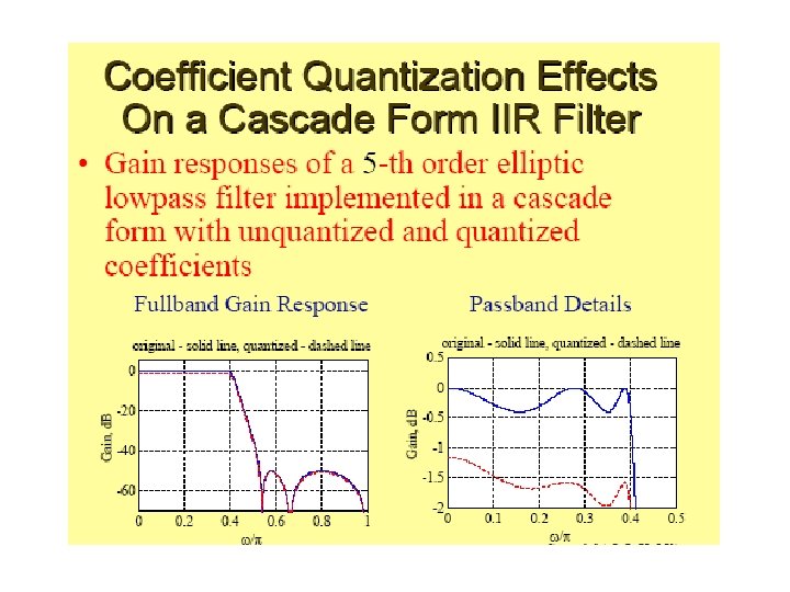
Realization Structures - Step 3 u Cascade structure - the transfer function can be factored into a cascade of a second order terms: u The difference equation of each stage: u This leads to the following structure…
 Cascade structure: A forth order IIR filter")
Realization Structures - Step 3 u x(n) Cascade structure: A forth order IIR filter with two direct form I sections in cascade y(n)

Analysis of Finite Wordlength Effects u u u The coefficients ak and bk of the designed filter are of an unlimited precision. However, when such a filter is implemented on a digital system (computer or dedicated hardware) of a small finite wordlength, errors arise in representing the filter coefficients and in performing the arithmetic operations indicated by the difference equation Before implementing an IIR filter, it is important to ascertain the extent to which its performance is degraded by a finite wordlength, and to make the required corrections, if the degradation is not acceptable

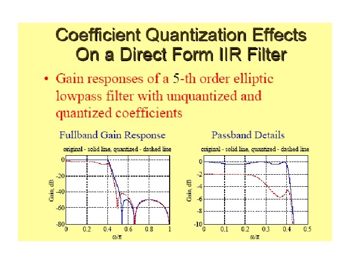
Analysis of Finite Wordlength Effects u The main errors in digital IIR filters are: w w ADC quantization noise, resulted from representing the samples of the input data by a small number of bits Coefficient quantization errors, caused by representing the IIR filter coefficients by a finite number of bits Overflow errors, which result from the arithmetic operations of filtering (multiplication and accumulation) using a limited register length Product round-off errors, caused when the output samples are truncated to the permissible wordlength

Analysis of Finite Wordlength Effects u The extent of filter degradation depends on w w w u u The wordlength and type of arithmetic used to perform the filtering The method used to quantize the filter coefficients The filter structure The user must analyze the effects of errors mentioned on the filter performance. The filter may become unstable, or its specifications altered

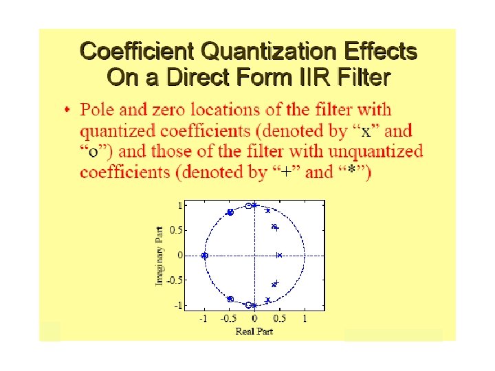
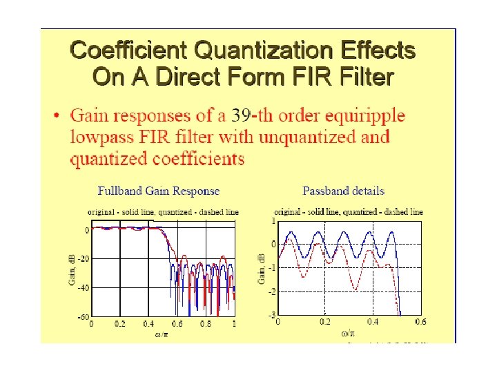
Coefficient Quantization Errors u u The primary effect of quantizing the filter coefficients into a finite number of bits is to alter the positions of the poles and zeros of H(z) in the zplane If, to start with, the filter poles are located near the unit circle, any significant deviation in their position could make the filter unstable As well as potential instability, deviations in the location of poles and zeroes also leads to the deviation of the filter from the desired frequency response The quantized filter should be analyzed to ensure that after quantization of its coefficient it is still stable and follows the desired frequency response

Overflow Error and Scaling u u In 2’s complement arithmetic, the addition of two (or more) large values may produce an overflow, that is a result that exceeds the permissible wordlength. Because of the recursive nature of IIR filters, an overflow at the output is fed back and used to compute the next output, causing further oveflow. To avoid or reduce the possibility of overflow, a scaling factor is used to scale down the input to the filter. Then, to keep the overall filter gain the same, the output is scaled up by the same factor

Product Roundoff Error u u The basic operation in IIR filtering involves the multiplication of the input samples by the coefficients bk, and the output samples by ak In practice, the samples and coefficients are commonly represented as fixed point numbers. The products bkx(n-k) and aky(n-k) is 2 B bits long, when the coefficients and samples are B bits long. For recursive filters, if this result is not reduced, subsequent computations will cause the number of bits to grow without limit

Product Roundoff Error u u Fortunately, such a problem is avoided in modern DSP processors These processors support double-wordlength accumulation. They include a built-in 16 x 16 bit multiplier, with 32 bit product register, and allow the products to be accumulated as 32 bit numbers Still, in practice, rounding or truncation at some point within the filter is required, to satisfy the wordlength requirements of the multiplier, data memory or interface with the outside world

ADC Quantization Noise u u The ADC quantizes the analogue input signal into a finite number of bits. This gives rise to quantization noise. The quantization error is uniformly distributed in the range [-D/2, D/2], where D is the quantization step With B quantization bits, D=2 -B , the quantization noise power, or variance, is The noise due to ADC quantization is fed into the IIR filer as an irreversible error
![IIR Filter Design Using MATLAB BUTTORD Butterworth filter order selection. [N, Wn] = BUTTORD(Wp,](http://slidetodoc.com/presentation_image_h/8101edd7b031e0a64123cf061c88e346/image-48.jpg "IIR Filter Design Using MATLAB BUTTORD Butterworth filter order selection. [N, Wn] = BUTTORD(Wp,")
IIR Filter Design Using MATLAB BUTTORD Butterworth filter order selection. [N, Wn] = BUTTORD(Wp, Ws, Rp, Rs) returns the order N of the lowest order digital Butterworth filter that loses no more than Rp d. B in the passband has at least Rs d. B of attenuation in the stopband. Wp and Ws are the passband stopband edge frequencies, normalized from 0 to 1 (where 1 corresponds to pi radians/sample). For example, Lowpass: Wp =. 1, Ws =. 2 Highpass: Wp =. 2, Ws =. 1 Bandpass: Wp = [. 2. 7], Ws = [. 1. 8] Bandstop: Wp = [. 1. 8], Ws = [. 2. 7] BUTTORD also returns Wn, the Butterworth natural frequency (or, the "3 d. B frequency") to use with BUTTER to achieve the specifications. [N, Wn] = BUTTORD(Wp, Ws, Rp, Rs, 's') does the computation for an analog filter, in which case Wp and Ws are in radians/second.
![IIR Filter Design Using MATLAB BUTTER Butterworth digital and analog filter design. [B, A]](http://slidetodoc.com/presentation_image_h/8101edd7b031e0a64123cf061c88e346/image-49.jpg "IIR Filter Design Using MATLAB BUTTER Butterworth digital and analog filter design. [B, A]")
IIR Filter Design Using MATLAB BUTTER Butterworth digital and analog filter design. [B, A] = BUTTER(N, Wn) designs an Nth order lowpass digital Butterworth filter and returns the filter coefficients in length N+1 vectors B (numerator) and A (denominator). The coefficients are listed in descending powers of z. The cutoff frequency Wn must be 0. 0 < Wn < 1. 0, with 1. 0 corresponding to half the sample rate. If Wn is a two-element vector, Wn = [W 1 W 2], BUTTER returns an order 2 N bandpass filter with passband W 1 < W 2. [B, A] = BUTTER(N, Wn, 'high') designs a highpass filter. [B, A] = BUTTER(N, Wn, 'stop') is a bandstop filter if Wn = [W 1 W 2].

IIR Filtering Using MATLAB % design an IIR low-pass filter with passband frequency of wp=800 Hz, % and attenuation of 20 db at frequency ws=1600 Hz , considering a sampling % frequency of fs=8000 Hz [x 1, fs]=wavread('c: tempbuchelli_res') ; wp=800/4000 ; ws=1600/4000 ; rp=1 ; rs=20 ; [N, wn]=buttord(wp, ws, rp, rs) ; [b, a]=butter(N, wn) ; freqz(b, a, 512, 8000) ; H=freqz(b, a, 512, 8000) ; %plot(abs(H)) x=x 1(10000: 30000) ; y=filter(b, a, x) ; % filtering using Matlab function figure(2) subplot(311), plot(x(10000: 10500)) subplot(312), plot(y(10000: 10500))
=0 ; for")
IIR Filtering Using MATLAB % filtering using the difference equation y(1: 4)=0 ; for i=length(b): length(x) sx=sum(b'. *x(i: -1: i-4)) ; sy=sum(a(2: length(a)). *y 1(i-1: i-4)) ; y(i)=sx-sy ; end subplot(312), plot(y 1(10000: 10500))].

IIR Filtering Using MATLAB fdatool Open a new session
")
IIR Filtering Using MATLAB fdatool Select IIR Filter and type (e. g. lowpass)

IIR Filtering Using MATLAB fdatool Select filter order, sampling frequency and cutoff frequency

IIR Filtering Using MATLAB fdatool Select Design Filter

IIR Filtering Using MATLAB fdatool Select Edit Convert Structure Direct Form I

IIR Filtering Using MATLAB fdatool Select Target Generate C Header Specify names and type

IIR Filter Design Using MATLAB fdatool u In case that the coefficients are to be modified, e. g. , when they have to be converted to integers, they have first to be exported to matlab workspace by File Export to Workspace Coefficients SOS and G u u u In the workplace, the a coefficients of the first stage are multiplied by the product of the stage gains Then they are multiplied by a constant (215) and rounded to integer. Following, they are imported back to fdatool using File Import Filter from Workspace u u Display the modified filter frequency response, and verify that it is close to the original (particularly the passing/stopping gains) The filter coefficients may be stored in a file or in an two coefficient arrays for a’s and b’s

IIR Filtering Using C and DSK // Low pass, Direct Form iir filter of order 5 // and a cutoff frequency of , , , -FP implementation #define Na 4 #define Nb 5 #define M 512 float samplex[Nb], sampley[Na] , ai[Na], bi[Nb] ; short sample_in[M], filt_array[M] ; float ai[Na]={-1. 9908, 1. 7650, -0. 7403, 0. 1235} ; float bi[Nb]={0. 0098, 0. 0393, 0. 0590, 0. 0393, 0. 0098} ; short i, j=0 ;
 //interrupt service routine {")
IIR Filtering Using C and DSK interrupt void c_int 11() //interrupt service routine { int sample_data, filt_samp ; float filt_sample=0. 0, filt_samplex=0, filt_sampley=0. 0 ; sample_data = input_sample() ; //input data // shift input data buffer for (i=Nb-2 ; i>=0 ; i--) samplex[i+1]=samplex[i] ; samplex[0]=(float)(sample_data) ; // filtering - 1 st stage for (i=0 ; i<Nb ; i++) filt_samplex += samplex[i]*bi[i] ; //filt_sample = ( filt_sample >> 15 ) ; //divide by 2^15 to get 16 bit samples // filtering - 2 nd stage for (i=0 ; i<Na ; i++) filt_sampley += sampley[i]*ai[i] ; filt_sample=filt_samplex-filt_sampley ;

IIR Filtering Using C and DSK // shift output data buffer for (i=Na-2 ; i>=0 ; i--) sampley[i+1]=sampley[i] ; sampley[0]=filt_sample ; filt_samp=(int)(filt_sample) ; output_sample(filt_samp); //output data filt_array[j]=filt_samp ; sample_in[j]=sample_data ; j++; if (j >= M) j=0; return; }
 { int i ; for (i=0")
IIR Filtering Using C and DSK void main() { int i ; for (i=0 ; i<Na ; i++) sampley[i]=0 ; for (i=0 ; i<Nb ; i++) samplex[i]=0 ; } comm_intr(); //init DSK, codec, Mc. BSP while(1); //infinite loop

IIR Filtering Using Cascade form on DSK //IIR filter using cascaded Direct Form II //Coefficients a's and b's correspond to b's and a's from MATLAB #define M 512 #include "DSK 6713_AIC 23. h" //codec-DSK support file Uint 32 fs=DSK 6713_AIC 23_FREQ_8 KHZ; //set sampling rate #include "lp 2000. cof" //LP @ 2000 Hz coefficient file //#include "bs 1750. cof" //BS @ 1750 Hz coefficient file //#include "bp 2000. cof" //BP @ 2000 Hz coefficient file short dly[stages][2] = {0}; //delay samples per stage short sample_in[M], filt_array[M] ; short j=0 ; void main() { comm_intr(); while(1); } / /init DSK, codec, Mc. BSP //infinite loop
 //ISR { short")
IIR Filtering Using Cascade form on DSK interrupt void c_int 11() //ISR { short i, input; int un, yn; input = input_sample(); //input to 1 st stage sample_in[j]=input ; for (i = 0; i < stages; i++) //repeat for each stage { un=input-((b[i][0]*dly[i][0])>>15) - ((b[i][1]*dly[i][1])>>15); yn=((a[i][0]*un)>>15)+((a[i][1]*dly[i][0])>>15)+((a[i][2]*dly[i][1])>>15); dly[i][1] = dly[i][0]; dly[i][0] = un; //update delays input = yn; //intermediate output->input to next stage } output_sample((short)yn); //output final result for time n filt_array[j]=(short)yn ; j++; if (j >= M) j=0; return; } //return from ISR

IIR Filtering Using Cascade form on DSK – Filter Coefficients File //lp 2000. cof IIR lowpass coefficients file, cutoff frequency 2 k. Hz #define stages 4 //number of 2 nd-order stages int a[stages][3] = { //numerator coefficients {304, 608, 304}, //a 10, a 11, a 12 for 1 st stage {32768, 66530, 33778}, //a 20, a 21, a 22 for 2 nd stage {32768, 65518, 32765}, //a 30, a 31, a 32 for 3 rd stage {32768, 64542, 31788} }; //a 40, a 41, a 42 for 4 th stage int b[stages][2] = //denominator coefficients { {0, 318}, //b 11, b 12 for 1 st stage {0, 3015}, //b 21, b 22 for 2 nd stage {0, 9362}, //b 31, b 32 for 3 rd stage {0, 22070} }; //b 41, b 42 for 4 th stage
- Slides: 65