Infinite Impulse Response IIR Filters Sometimes called recursive

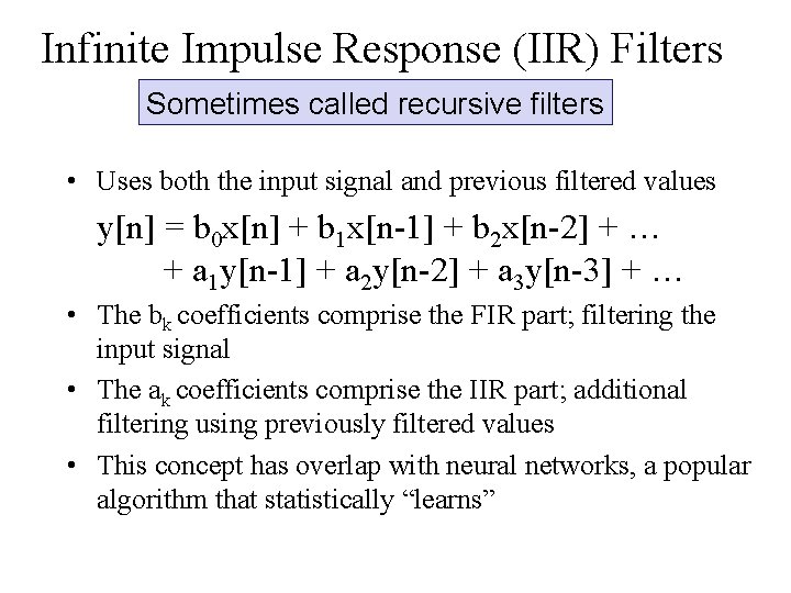
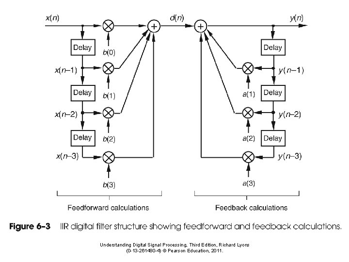
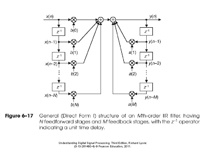
Infinite Impulse Response (IIR) Filters Sometimes called recursive filters • Uses both the input signal and previous filtered values y[n] = b 0 x[n] + b 1 x[n-1] + b 2 x[n-2] + … + a 1 y[n-1] + a 2 y[n-2] + a 3 y[n-3] + … • The bk coefficients comprise the FIR part; filtering the input signal • The ak coefficients comprise the IIR part; additional filtering using previously filtered values • This concept has overlap with neural networks, a popular algorithm that statistically “learns”

IIR Filter Code public static double[] convolution(double[] signal, double[] b, double[] a) { double[] y = new double[signal. length + b. length - 1]; for (int i = 0; i < signal. length; i ++) { for (int j = 0; j < b. length; j++) { if (i-j>=0) y[i] += b[j]*signal[i - j]; } if (a!=null) { for (int j = 1; j < a. length; j ++) { if (i-j>=0) y[i] -= a[j] * y[i - j]; } } } return y; }

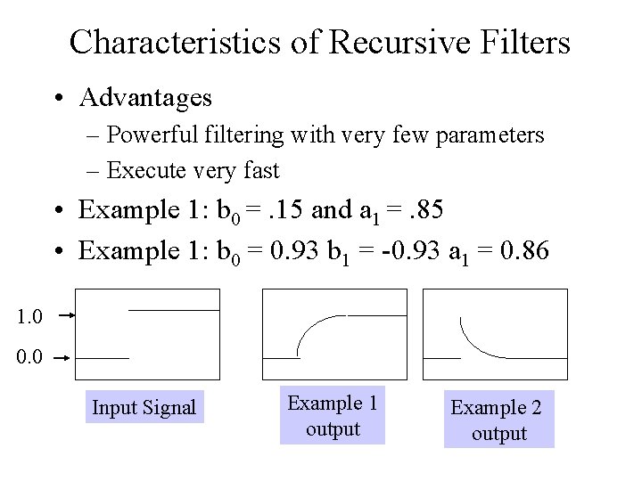
Characteristics of Recursive Filters • Advantages – Powerful filtering with very few parameters – Execute very fast • Example 1: b 0 =. 15 and a 1 =. 85 • Example 1: b 0 = 0. 93 b 1 = -0. 93 a 1 = 0. 86 1. 0 0. 0 Input Signal Example 1 output Example 2 output

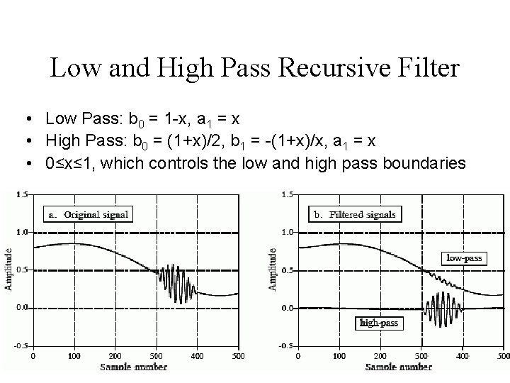
Low and High Pass Recursive Filter • Low Pass: b 0 = 1 -x, a 1 = x • High Pass: b 0 = (1+x)/2, b 1 = -(1+x)/x, a 1 = x • 0≤x≤ 1, which controls the low and high pass boundaries

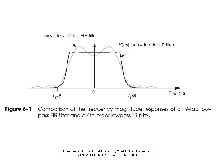
Understanding Digital Signal Processing, Third Edition, Richard Lyons (0 -13 -261480 -4) © Pearson Education, 2011.

Understanding Digital Signal Processing, Third Edition, Richard Lyons (0 -13 -261480 -4) © Pearson Education, 2011.

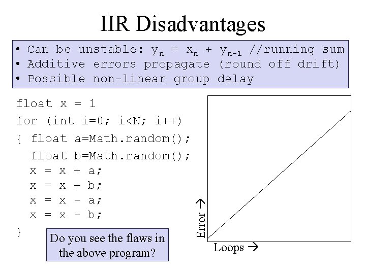
IIR Disadvantages float x = 1 for (int i=0; i<N; i++) { float a=Math. random(); float b=Math. random(); x = x + a; x = x + b; x = x - a; x = x - b; } Do you see the flaws in the above program? Error • Can be unstable: yn = xn + yn-1 //running sum • Additive errors propagate (round off drift) • Possible non-linear group delay Loops

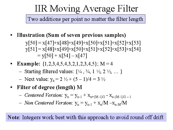
IIR Moving Average Filter Two additions per point no matter the filter length • Illustration (Sum of seven previous samples) y[50] = x[47]+x[48]+x[49]+x[50]+x[51]+x[52]+x[53] y[51] = x[48]+x[49]+x[50]+x[51]+x[52]+x[53]+x[54] = y[50] + x[54] – x[47] • Example: {1, 2, 3, 4, 5, 4, 3, 2, 1, 2, 3, 4, 5}; M = 4 – Starting filtered values: {¼ , ¾, 1 ½, 2 ½, … } – Next value: y 4 = 2 ½ + (5 – 1)/4 = 3 ½ • Filter of degree (length) M – Centered Version: yn = yn-1 + xn+(M-1)/2 - xn-(M-1)/2 – 1 – Non Centered Version: yn = yn-1 + xn/M –xn-M/M Note: Integers work best with this approach to avoid round off drift

Transforms Some problems are difficult (or impossible) to solve directly • Procedure – Transform the problem into a different domain – Execute a simpler algorithm in the transformed space – Transform back to get the solution • DSP Example: We need a well-defined way to determine IIR filter coefficients that result in a filter that performs properly • Image Processing: Mapping a three dimensional image into two dimension

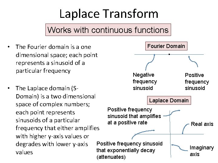
Laplace Transform Works with continuous functions • The Fourier domain is a one dimensional space; each point represents a sinusoid of a particular frequency . Fourier Domain Negative frequency sinusoid Positive frequency sinusoid • The Laplace domain (SDomain) is a two dimensional Laplace Domain space of complex numbers; Positive frequency each point represents sinusoid that amplifies sinusoids of a particular at a positive rate Real axis frequency that either amplifies with higher y-axis values or degrades with lower y-axis Positive frequency sinusoid Imaginary that exponentially decay values axis (attenuates)

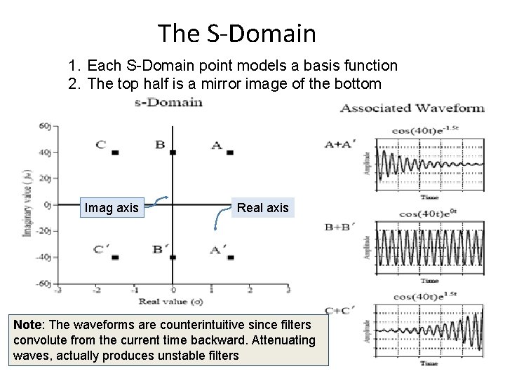
The S-Domain 1. Each S-Domain point models a basis function 2. The top half is a mirror image of the bottom Imag axis Real axis Note: The waveforms are counterintuitive since filters convolute from the current time backward. Attenuating waves, actually produces unstable filters

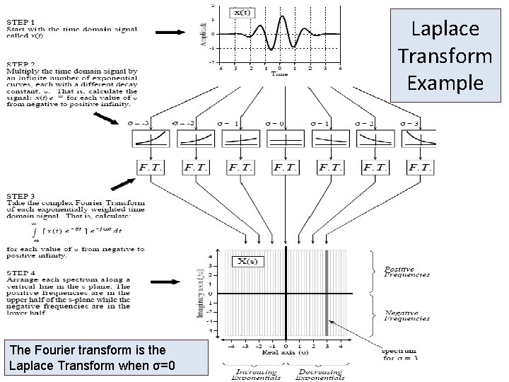
Laplace Transform Example The Fourier transform is the Laplace Transform when σ=0

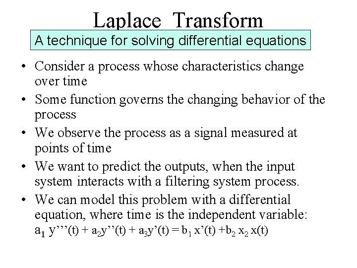
Laplace Transform A technique for solving differential equations • Consider a process whose characteristics change over time • Some function governs the changing behavior of the process • We observe the process as a signal measured at points of time • We want to predict the outputs, when the input system interacts with a filtering system process. • We can model this problem with a differential equation, where time is the independent variable: a 1 y’’’(t) + a 2 y’’(t) + a 3 y’(t) = b 1 x’(t) +b 2 x(t)

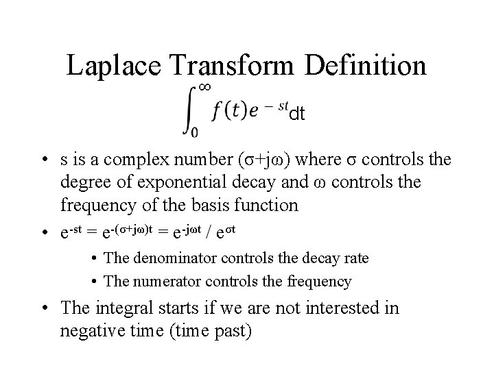
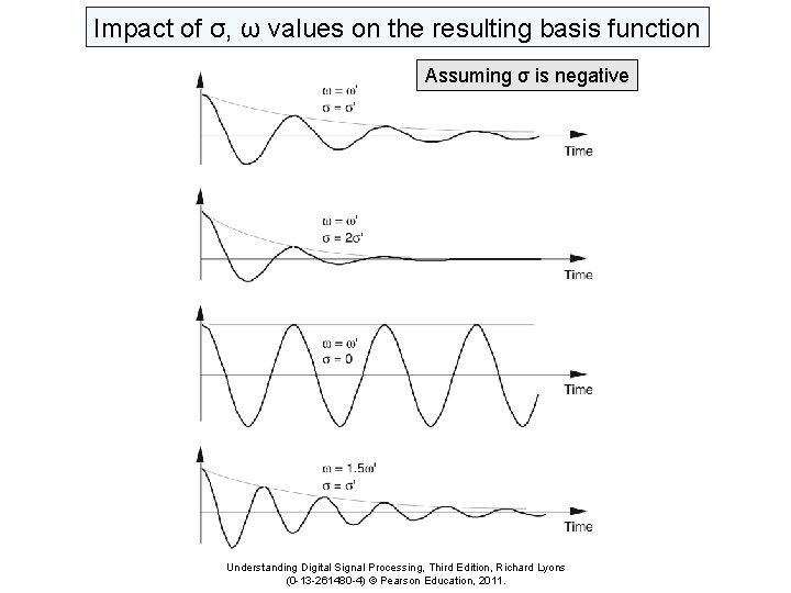
Laplace Transform Definition dt • s is a complex number (σ+jω) where σ controls the degree of exponential decay and ω controls the frequency of the basis function • e-st = e-(σ+jω)t = e-jωt / eσt • The denominator controls the decay rate • The numerator controls the frequency • The integral starts if we are not interested in negative time (time past)

Impact of σ, ω values on the resulting basis function Assuming σ is negative Understanding Digital Signal Processing, Third Edition, Richard Lyons (0 -13 -261480 -4) © Pearson Education, 2011.

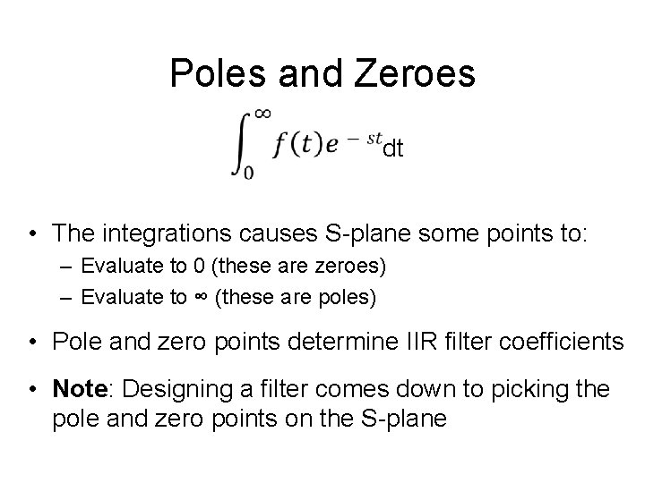
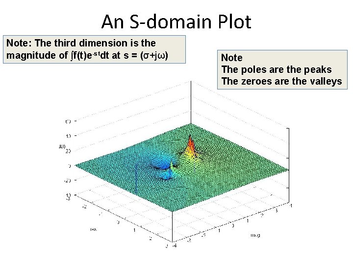
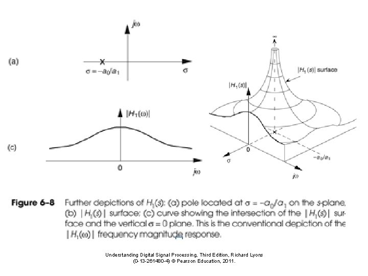
Poles and Zeroes dt • The integrations causes S-plane some points to: – Evaluate to 0 (these are zeroes) – Evaluate to ∞ (these are poles) • Pole and zero points determine IIR filter coefficients • Note: Designing a filter comes down to picking the pole and zero points on the S-plane

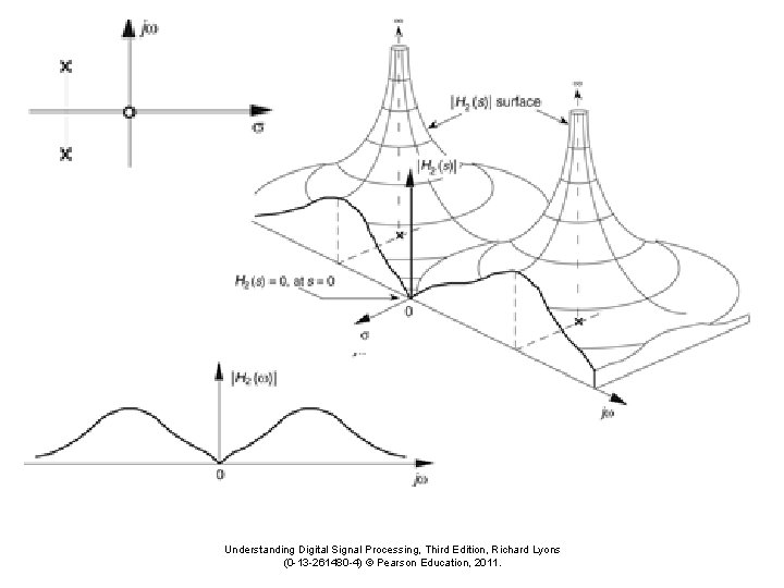
An S-domain Plot Note: The third dimension is the magnitude of ∫f(t)e-stdt at s = (σ+jω) Note The poles are the peaks The zeroes are the valleys

Understanding Digital Signal Processing, Third Edition, Richard Lyons (0 -13 -261480 -4) © Pearson Education, 2011.

Understanding Digital Signal Processing, Third Edition, Richard Lyons (0 -13 -261480 -4) © Pearson Education, 2011.

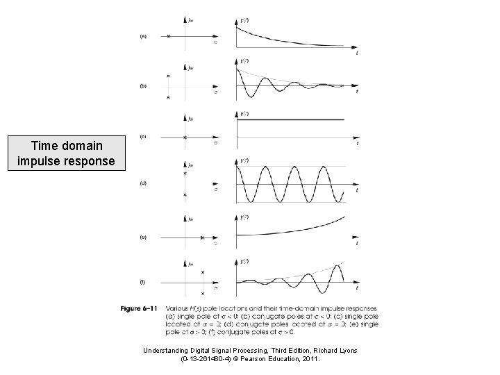
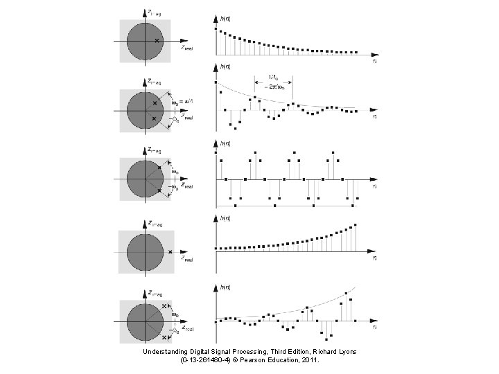
Time domain impulse response Understanding Digital Signal Processing, Third Edition, Richard Lyons (0 -13 -261480 -4) © Pearson Education, 2011.

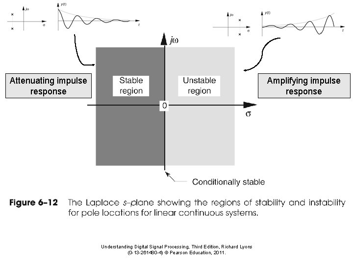
Attenuating impulse response Amplifying impulse response Understanding Digital Signal Processing, Third Edition, Richard Lyons (0 -13 -261480 -4) © Pearson Education, 2011.

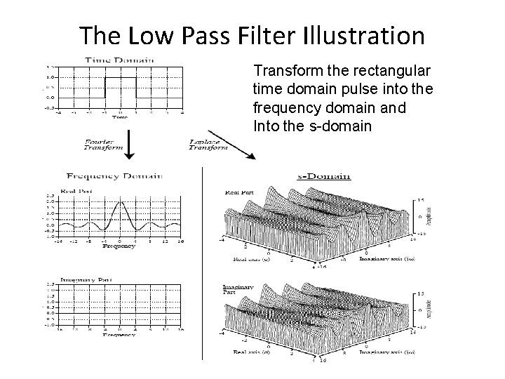
The Low Pass Filter Illustration Transform the rectangular time domain pulse into the frequency domain and Into the s-domain

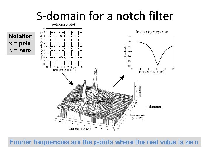
S-domain for a notch filter Notation x = pole ○ = zero Fourier frequencies are the points where the real value is zero

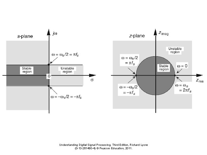
The z-transform Z{x[n]} = • Z-transform is the discrete cousin to the Laplace Transform • Laplace Transform (s = σ+jω) – – Extends the Fourier Transform, uses integrals and continuous functions s = e-(σ+jω)t becomes the Fourier transform when ω = 0 Fourier points fall along the imaginary axis S-domain stable region is on the negative half of the domain • Z-Transform (z = re-2πk/ts) – – Extends the Discrete Fourier Transform, uses sums and discrete samples z = e-j 2πk/ts becomes the Discrete Fourier Transform (ts=sample size) Four transform points fall along the unit circle Z-domain stable domain are those within the unit circle

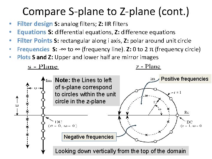
Compare S-plane to Z-plane (cont. ) • Filter design S: analog filters; Z: IIR filters • Equations S: differential equations, Z: difference equations • Filter Points S: rectangular along i axis, Z: polar around unit circle • Frequencies S: -∞ to ∞ (frequency line). Z: 0 to 2 π (frequency circle) • Plots S and Z: Upper and lower half are mirror images Note: the Lines to left of s-plane correspond to circles within the unit circle in the z-plane Positive frequencies Negative frequencies Looking down vertically from the top of the domain

Understanding Digital Signal Processing, Third Edition, Richard Lyons (0 -13 -261480 -4) © Pearson Education, 2011.

Understanding Digital Signal Processing, Third Edition, Richard Lyons (0 -13 -261480 -4) © Pearson Education, 2011.

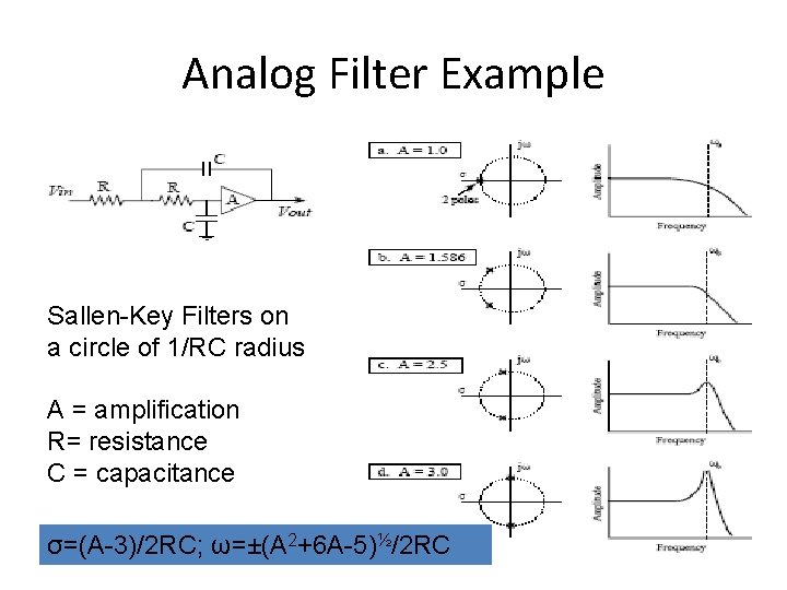
Analog Filter Example Sallen-Key Filters on a circle of 1/RC radius A = amplification R= resistance C = capacitance σ=(A-3)/2 RC; ω=±(A 2+6 A-5)½/2 RC

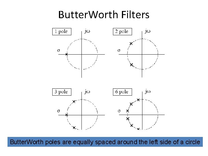
Butter. Worth Filters Butter. Worth poles are equally spaced around the left side of a circle

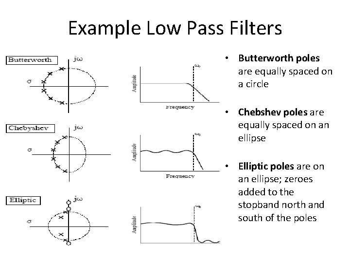
Example Low Pass Filters • Butterworth poles are equally spaced on a circle • Chebshev poles are equally spaced on an ellipse • Elliptic poles are on an ellipse; zeroes added to the stopband north and south of the poles

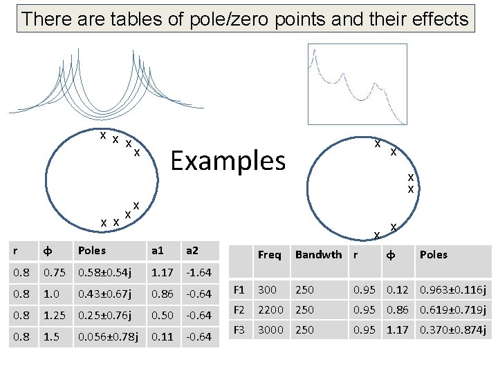
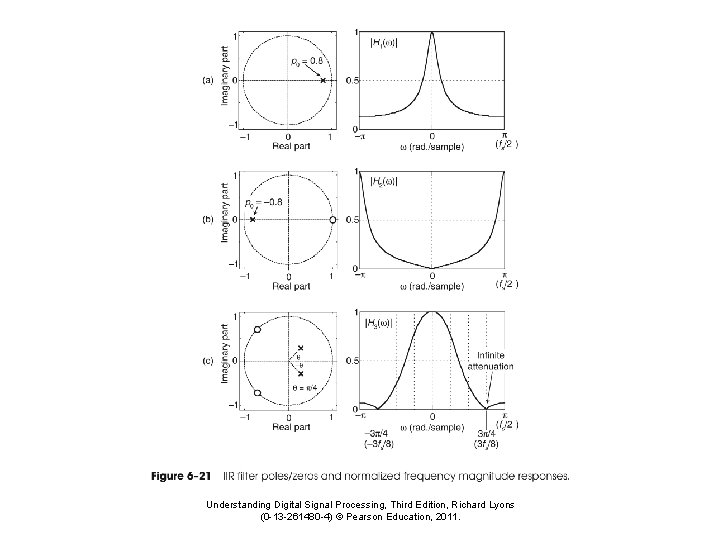
There are tables of pole/zero points and their effects x x x x Examples x x x r φ Poles a 1 a 2 0. 8 0. 75 0. 58± 0. 54 j 1. 17 -1. 64 0. 8 1. 0 0. 43± 0. 67 j 0. 86 -0. 64 0. 8 1. 25 0. 25± 0. 76 j 0. 50 -0. 64 0. 8 1. 5 0. 056± 0. 78 j 0. 11 -0. 64 x Freq Bandwth r φ Poles F 1 300 250 0. 95 0. 12 0. 963± 0. 116 j F 2 2200 250 0. 95 0. 86 0. 619± 0. 719 j F 3 3000 250 0. 95 1. 17 0. 370± 0. 874 j

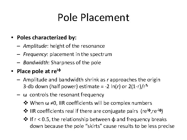
Pole Placement • Poles characterized by: – Amplitude: height of the resonance – Frequency: placement in the spectrum – Bandwidth: Sharpness of the pole • Place pole at reiφ – Amplitude and bandwidth shrink as r approaches the origin 3 -db down (half power) estimate = -2 ln(r) or 2(1 -r)/r½ – ω controls the resonant frequency v When ω ≠ 0, IIR coefficients will be complex numbers v IIR coefficients real if there are conjugate pairs (reiφ, re-iφ) v If r < 0. 5, the relationship between φ and frequency breaks down because the pole “skirts” cause results to be less precise

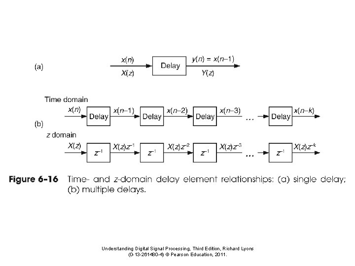
Transfer Function Z{x[n]} = 1. 2. 3. 4. 5. 6. 7. A polynomial equation that defines filter coefficients for particular Z, S domain setting IIR Definition: yn = b 0 xn + b 1 xn-1 +…+ b. Mxn-M + a 1 yn-1 +…+ a. Nyn-N Z transform both sides: Yz=Z{b 0 xn+b 1 xn-1+…+b. Mxn-M+a 1 yn-1+…+a. Nyn-N} Linearity Property: Yz = Z{b 0 xn}+Z{b 1 xn-1}+…+Z{b. Mxn-M}+Z{a 1 yn-1}+…+Z{a. Nyn-N} Time delay property (Z{xn-k} = xzz-k) Yz = b 0 Xz + b 1 Xzz-1 +…+bn-MXzz-M + a 1 Yzz-1+…+a. NYzz-N Gather Terms Yz - a 1 Yzz-1 -…- a. NYzz-N = b 0 Xz + b 1 Xzz-1 +…+ bn-MXz-M Yz(1 - a 1 z-1 -…- a. Nz-N ) = Xz(b 0 + b 1 z-1 +…+ bn-Mz-M) Divide to get transfer function Yz/Xz= Hz= (b 0 + b 1 z-1 +…+ bn-Mz-M)/(1 - a 1 z-1 -…- a. Nz-N ) Yz = Xz (Yz/Xz) = Xz (Hz) // Hz is the transform function for the filter Perform Inverse Z transform: y[n] = x[n] * filter[n] // where * is convolution Because Z domain multiplication is time domain convolution Starting with the IIR definition, derive Z-Transform Transfer Function

Understanding Digital Signal Processing, Third Edition, Richard Lyons (0 -13 -261480 -4) © Pearson Education, 2011.

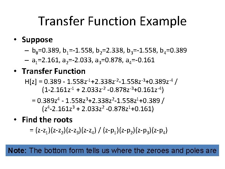
Transfer Function Example • Suppose – b 0=0. 389, b 1=-1. 558, b 2=2. 338, b 3=-1. 558, b 4=0. 389 – a 1=2. 161, a 2=-2. 033, a 3=0. 878, a 4=-0. 161 • Transfer Function H[z] = 0. 389 - 1. 558 z-1+2. 338 z-2 -1. 558 z-3+0. 389 z-4 / (1 -2. 161 z-1 + 2. 033 z-2 -0. 878 z-3+0. 161 z-4) = 0. 389 z 4 - 1. 558 z 3+2. 338 z 2 -1. 558 z 1+0. 389 / (z 4 -2. 161 z 3 + 2. 033 z 2 -0. 878 z 1+0. 161) • Find the roots = (z-z 1)(z-z 2)(z-z 3)(z-z 4) / (z-p 1)(z-p 2)(z-p 3)(z-p 4) Note: The bottom form tells us where the zeroes and poles are

Understanding Digital Signal Processing, Third Edition, Richard Lyons (0 -13 -261480 -4) © Pearson Education, 2011.

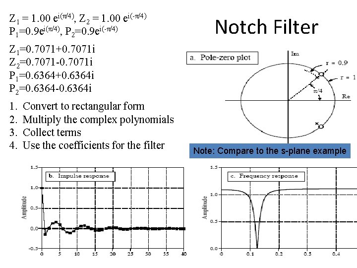
Z 1 = 1. 00 ei(π/4), Z 2 = 1. 00 ei(-π/4) P 1=0. 9 ei(π/4), P 2=0. 9 ei(-π/4) Notch Filter Z 1=0. 7071+0. 7071 i Z 2=0. 7071 -0. 7071 i P 1=0. 6364+0. 6364 i P 2=0. 6364 -0. 6364 i 1. 2. 3. 4. Convert to rectangular form Multiply the complex polynomials Collect terms Use the coefficients for the filter Note: Compare to the s-plane example

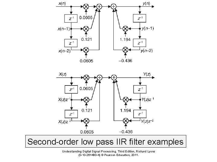
Second-order low pass IIR filter examples Understanding Digital Signal Processing, Third Edition, Richard Lyons (0 -13 -261480 -4) © Pearson Education, 2011.

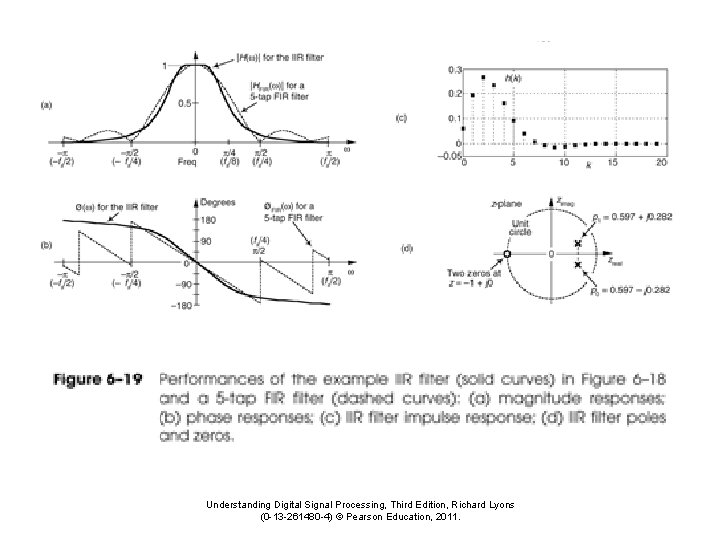
Understanding Digital Signal Processing, Third Edition, Richard Lyons (0 -13 -261480 -4) © Pearson Education, 2011.

Understanding Digital Signal Processing, Third Edition, Richard Lyons (0 -13 -261480 -4) © Pearson Education, 2011.

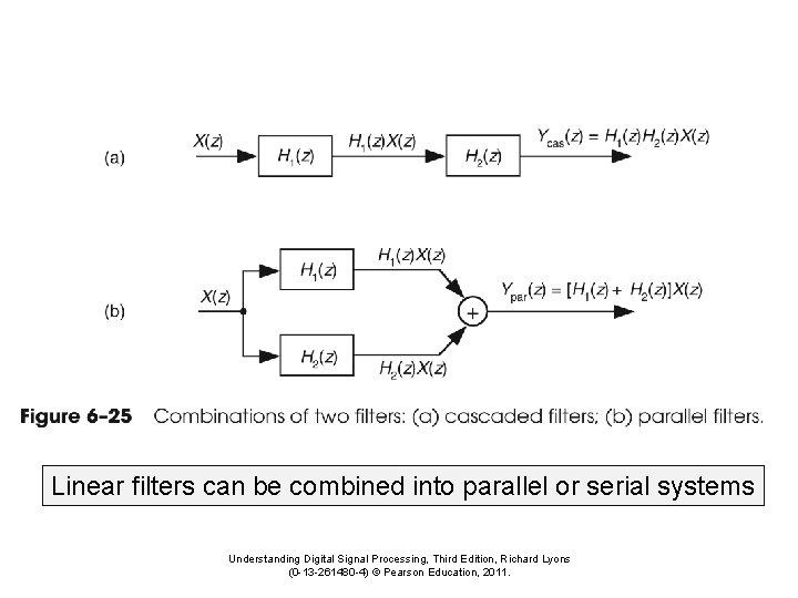
Linear filters can be combined into parallel or serial systems Understanding Digital Signal Processing, Third Edition, Richard Lyons (0 -13 -261480 -4) © Pearson Education, 2011.

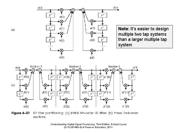
Note: It’s easier to design multiple two tap systems than a larger multiple tap system Understanding Digital Signal Processing, Third Edition, Richard Lyons (0 -13 -261480 -4) © Pearson Education, 2011.

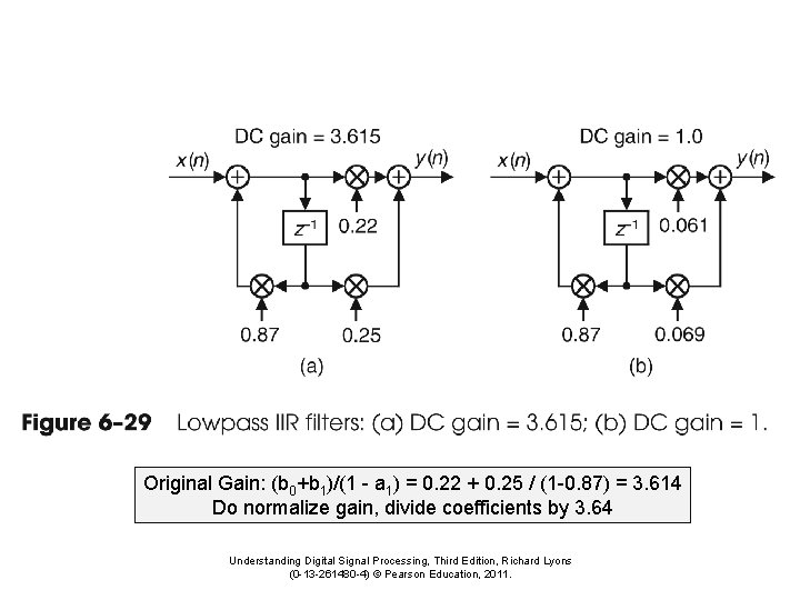
Original Gain: (b 0+b 1)/(1 - a 1) = 0. 22 + 0. 25 / (1 -0. 87) = 3. 614 Do normalize gain, divide coefficients by 3. 64 Understanding Digital Signal Processing, Third Edition, Richard Lyons (0 -13 -261480 -4) © Pearson Education, 2011.