2 2 Transfer function and impulseresponse function 2

2 -2 Transfer function and impulse-response function 2. Transfer function input x(t) output LTI system y(t) Definition: The transfer function of a linear timeinvariant system is defined as the ratio of the Laplace transform of the output variable to the Laplace transform of the input variable when all initial conditions are zero.

Consider the linear time-invariant system described by the following differential equation: By definition, the transfer function is

The advantage of transfer function: It represents system dynamics by algebraic equations and clearly shows the input-output relationship: Y(s)=G(s)X(s) input x(t) output G(s) y(t) Example. Given a system described by the following differential equation Find its transfer function.

Example. Spring-mass-damper system: Wall friction, b k y Let the input be the force r(t) and the output be the displacement y(t) of the mass. Find its transfer function. Solution: The system differential equation is r(t) Force from which we obtain its transfer function

Comments on transfer function: • is limited to LTI systems. • is an operator to relate the output variable to the input variable of a differential equation. • is a property of a system itself, independent of the magnitude and nature of the input or driving function. • does not provide any information concerning the physical structure of the system. That is, the transfer functions of many physically different systems can be identical.

Wall friction, b k y r(t) Force

3. Convolution integral From and by using the convolution theorem, we have where both g(t) and x(t) are 0 for t<0.

Example. Given with T >0. If R(s)=1/s, find y(t). Solution: By the definition of convolution integral, Hence, 1 t

4. Impulse response function Consider the output (response) of a system to a unit-impulse input when the initial conditions are zero: input (t) output G(s) y(t) Hence, and where g(t) is called impulse response function.

An impulse response function g(t) is the inverse Laplase transform of the system’s transfer function! Example. Given y (t) t R(s) Y(s) If determine the system’s transfer function. t

It is hence possible to obtain complete information about the dynamic characteristics of the system by exciting it with an impulse input and measuring the response (In practice, a pulse input with a very short duration can be considered an impulse). Example. Let y 1 (t) t R(s) Y(s) e-t 2 1 Assume that the system is LTI. Determine its transfer function. t

Example. Let Determine its impulse response function.

2 -3 Automatic control systems 1. Block Diagrams l Block diagram of a system is a pictorial representation of the functions performed by each component and of the flow of signals. R C G(s) or

2. Block Diagram of a closed-loop system A real physical system includes more than one components. The following is a typical feedback system represented by block diagram: E R(s) B(s) G(s) C(s) H(s) where the summing point E(s)=R(s) B(s) and the branch point are shown below. E Y(s) R(s) B(s) Y(s)

The property of summing point:

Example. A network system is shown below, where uc is the output and ur is the input. Draw its block diagram. Solution: Sept 1. Write the input and output relationship of each device: ur uc

Sept 2. Taking Laplace transform of both sides of the above equations yields: Sept 3. Rearrange each above equation so that its lefthand side is the output variable and the right-hand side is the transfer function multiplied by input signals:

Step 4. Based on (1)-(3), draw the block diagram:

Example. A system is described by the following equations: Draw its block diagram, where , Ki and T are positive constants, the input and output signals are r and c, respectively, and x 1 x 5 are intermediate variables. . r c

Example. A system is described by the following equations: Draw its block diagram, where Ki and T are positive constants, the input and output signals are r and c, respectively, n 1, n 2 are disturbances, and x 1 x 5 are intermediate variables. n 1 r n 2 c

3. Open-loop transfer function and feedforward transfer function E R(s) B(s) G(s) C(s) H(s) Two important concepts: Open-loop transfer function: The ratio of the feedback signal B(s) to the actuating error signal E(s) is called the open-loop transfer function. That is,

E R(s) B(s) G(s) C(s) H(s) Feedforward transfer function: The ratio of the output C(s) to the actuating error signal E(s) is called the feedforward transfer function, so that

4. Closed-loop transfer function E R(s) B(s) G(s) C(s) H(s) Substituting (2) into (2) yields from which we obtain the closed-loop transfer function as

Example. A block diagram of a system is shown below. Determine its closed-loop transfer function C(s)/R(s).

5. Obtaining cascaded, parallel, and feedback transfer functions a) Cascaded system R(s) G 1(s) U G 1(s)G 2(s) C(s)

Example. A block diagram of DC motor is shown below. Determine its open-loop transfer function and feedforward transfer function.

b) Parallel Blocks R(s) C(s) G 1(s) G 2(s) R(s) C(s)

c) Feedback loop E R(s) G C(s) H R(s) C(s)

Diagram simplification: Moving a summing point ahead of a block:

Diagram simplification : Moving a summing point behind a block:

Example. Simplify the following block diagram. Then obtain the closed-loop transfer function Eo(s)/Ei(s). If there exists a branch point between two summing points, do not move summing point.

Diagram simplification: Moving a branch point ahead of a block

Diagram simplification: Moving a branch point behind of a block

Example. Simplify the following block diagram. Then obtain the closed-loop transfer function Eo(s)/Ei(s).

Diagram simplification: Examples Example. The block diagram of a given system is shown below. Obtain C(s)/R(s). Note that only the movement between two summing points (two branch points) is valid.

Example. The block diagram of a given system is shown below. Obtain C(s)/R(s). If there exists a branch point (summing point) between two summing points (two branch points), do not move them.

Example. The block diagram of a given system is shown below. Obtain the transfer function that relates the output C(s) in function of the input R(s), i. e. , C(s)/R(s). G 3 R(s) G 2 G 1 C(s) H 1 Note that only the movement between two summing points (two branch points) is valid.

R(s) G 3 G 1 C(s) G 2 H 1 R(s) G 3 G 1 G 2 G 1 H 1 C(s)

An alternative way to simplify the diagram is G 3 G 1 1/G 1 G 3 G 1 G 2 H 1

Example. The block diagram of a given system is shown below. Obtain C(s)/R(s).

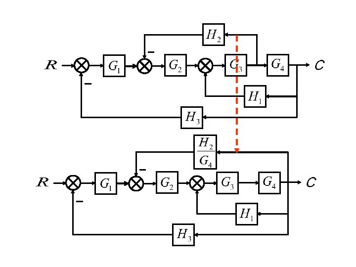
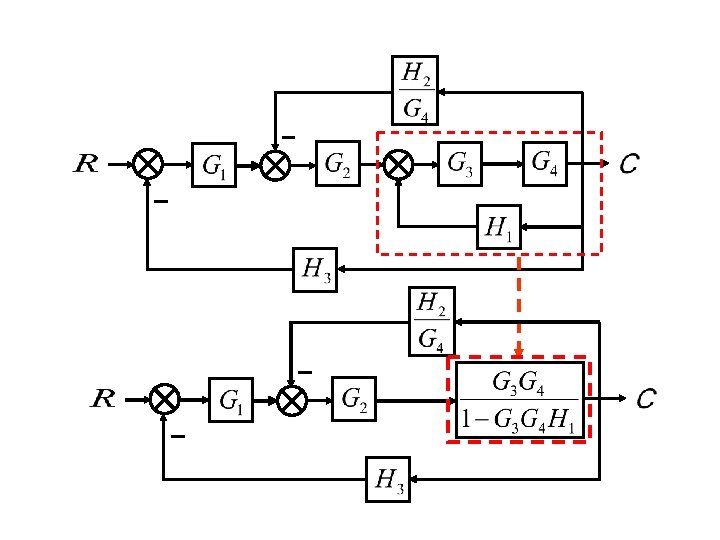
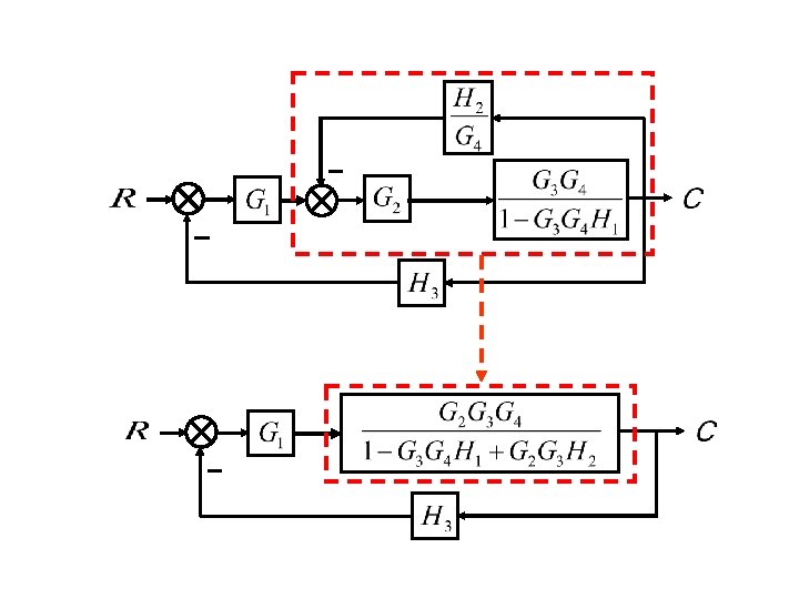
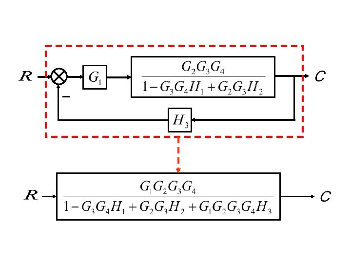
Example. Block reduction: Redrawing block diagram. Consider the following diagram. With redrawing the diagram, the simplification can be proceeded. G 4 G 1 H 1 G 2 G 3 H 3

G 4 G 1 G 2 G 3 H 1 H 3

Example. The block diagram of a system is shown below. Obtain C(s)/R(s).

5. The Mason’ Formula (supplement material) • = the characteristic polynomial of the system =1 Li+ Li. Lj. Lk+ ; • Li=transfer function of the ith loop; • Li. Lj=product of transfer functions of two nontouching loops; • Li. Lj. Lk=product of transfer functions of three nontouching loops; • Li. Lj. Lk. Ll…. . ;

• N=total number of forward paths (from R(s) to C(s) without visiting a point more than once); • Pk=transfer function of kth forward path; • k= the cofactor of the kth forward path with the loops touching the kth forward path removed.

Example. Determine the characteristic polynomial of the following block diagram:

Example. The block diagram of a given system is shown below. Determine its characteristic poly-nomial, forward paths and cofactors.

Example. For the following block diagram, find C(s)/R(s). Solution: By using Mason’s formula,

Only one forward path: Four individual loops: No nontouching loops, therefore, The cofactor is: Consequently,

6. Closed-loop systems subjected to a disturbance By principle of superposition, let, respectively, R(s)=0 and D(s)=0 and calculate the corres-ponding outputs CD(s) and CR(s). Then, C= CD(s) +CR(s) D R(s) G 2(s) G 1(s) H(s) C(s)

Example. The block diagram of a given system is shown below. Obtain C(s)/R(s) and C(s)/D(s).

Summary of Chapter 2 In this chapter, we mainly studied the following issues: 1. Laplace transformation and the related theorems. 2. Transfer function:

from which we know that • C(s)=G(s)R(s); • In time domain, the above equation represents a convolution integral: where g(t)= 1[G(s)]. • In particular, if r(t)= (t), c(t)= 1[G(s)], that is, the impulse response is the inverse Laplase transform of its transfer function.

3. Block diagram: Note that only one block is less meaning. However, with a block diagram, the interrelationship between components and the signal flows can be revealed pictorially compared with the mathematical expression of a set of equations; for instance:

4. Block diagram simplification (reduction): • feedback; • cascade; • parallel; • moving between two summing (branch) points; • redrawing the block diagram for some special cases.

By using diagram simplification techniques, one can finally obtain, no matter how complex a system may be, Cr(s)=G(s)R(s); Cd(s)= (s)D(s). Based on which, system analysis can be proceeded.