EEEcon 458 SCUC J Mc Calley 1 Unit

EE/Econ 458 SCUC J. Mc. Calley 1

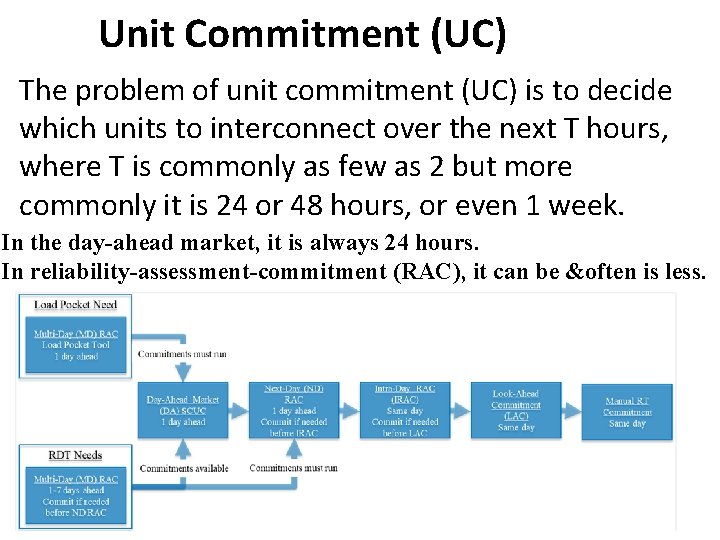
Unit Commitment (UC) The problem of unit commitment (UC) is to decide which units to interconnect over the next T hours, where T is commonly as few as 2 but more commonly it is 24 or 48 hours, or even 1 week. In the day-ahead market, it is always 24 hours. In reliability-assessment-commitment (RAC), it can be &often is less. 2

Unit Commitment (UC) The problem becomes security constrained (SCUC) when constraints are imposed to ensure line flows do not exceed chosen limits following a contingency. 3

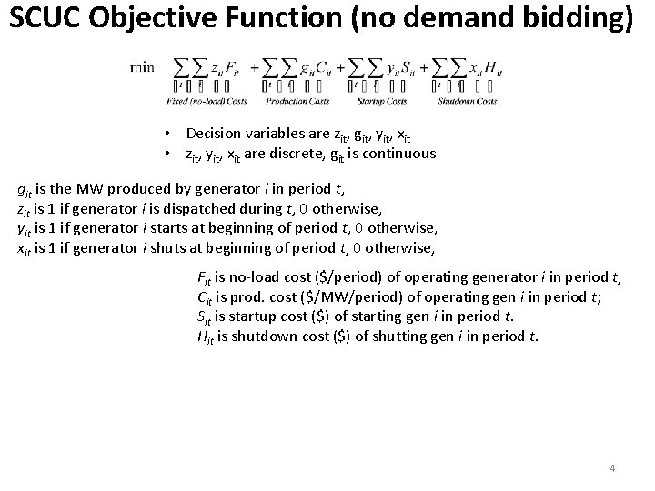
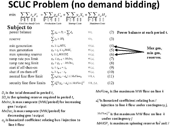
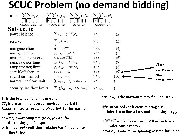
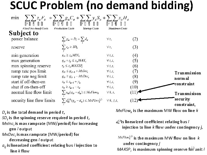
SCUC Objective Function (no demand bidding) • Decision variables are zit, git, yit, xit • zit, yit, xit are discrete, git is continuous git is the MW produced by generator i in period t, zit is 1 if generator i is dispatched during t, 0 otherwise, yit is 1 if generator i starts at beginning of period t, 0 otherwise, xit is 1 if generator i shuts at beginning of period t, 0 otherwise, Fit is no-load cost ($/period) of operating generator i in period t, Cit is prod. cost ($/MW/period) of operating gen i in period t; Sit is startup cost ($) of starting gen i in period t. Hit is shutdown cost ($) of shutting gen i in period t. 4

SCUC Problem (no demand bidding) Subject to Power balance at each period t. Max gen, min gen, reserves. Dt is the total demand in period t, SDt is the spinning reserve required in period t, Mx. Inci is max ramprate (MW/period) for increasing gen i output Mx. Deci is max ramprate (MW/period) for decreasing gen i output aij is linearized coefficient relating bus i injection to line k flow Mx. Flowk is the maximum MW flow on line k is linearized coefficient relating bus i injection to line k flow under contingency j, is the maximum MW flow on line k under contingency j MAXSPi is maximum spinning reserve for 5 unit i

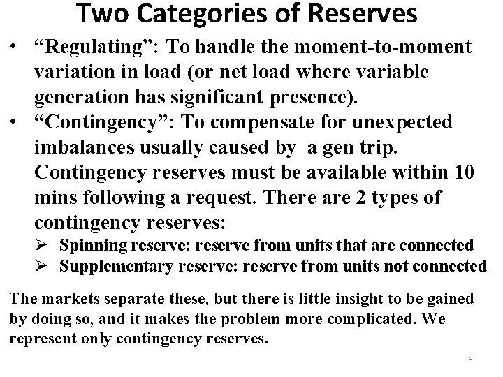
Two Categories of Reserves • “Regulating”: To handle the moment-to-moment variation in load (or net load where variable generation has significant presence). • “Contingency”: To compensate for unexpected imbalances usually caused by a gen trip. Contingency reserves must be available within 10 mins following a request. There are 2 types of contingency reserves: Ø Spinning reserve: reserve from units that are connected Ø Supplementary reserve: reserve from units not connected The markets separate these, but there is little insight to be gained by doing so, and it makes the problem more complicated. We represent only contingency reserves. 6

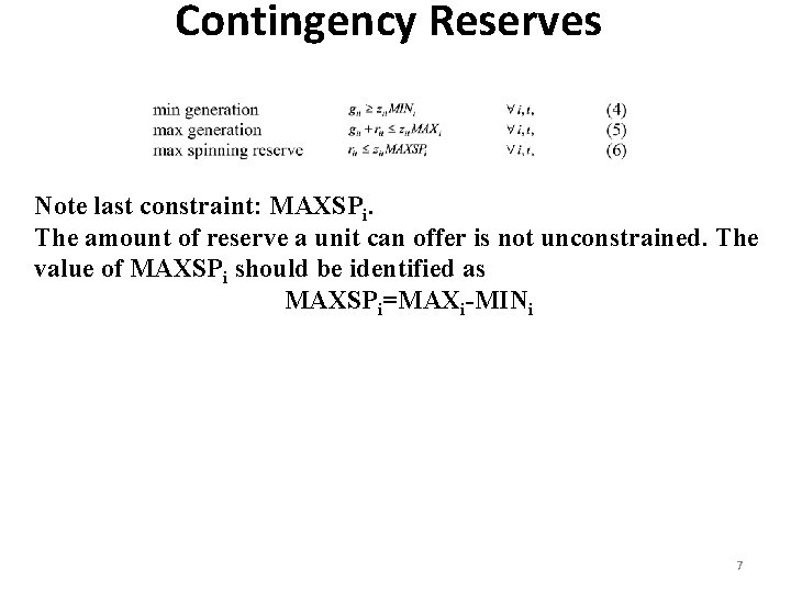
Contingency Reserves Note last constraint: MAXSPi. The amount of reserve a unit can offer is not unconstrained. The value of MAXSPi should be identified as MAXSPi=MAXi-MINi 7

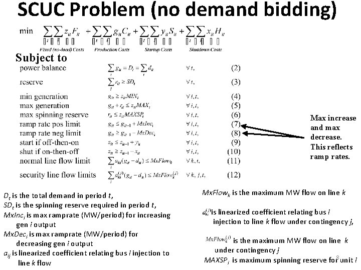
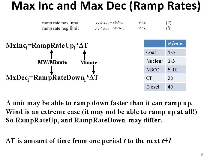
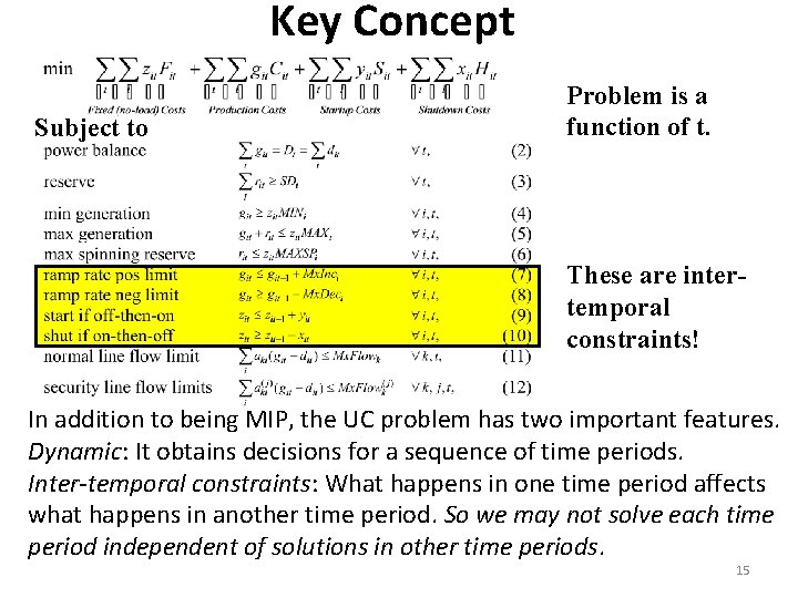
SCUC Problem (no demand bidding) Subject to Max increase and max decrease. This reflects ramp rates. Dt is the total demand in period t, SDt is the spinning reserve required in period t, Mx. Inci is max ramprate (MW/period) for increasing gen i output Mx. Deci is max ramprate (MW/period) for decreasing gen i output aij is linearized coefficient relating bus i injection to line k flow Mx. Flowk is the maximum MW flow on line k is linearized coefficient relating bus i injection to line k flow under contingency j, is the maximum MW flow on line k under contingency j MAXSPi is maximum spinning reserve for 8 unit i

Max Inc and Max Dec (Ramp Rates) Mx. Inci=Ramp. Rate. Upi*ΔT MW/Minute Mx. Deci=Ramp. Rate. Downi*ΔT %/min Coal 1 -5 Nuclear 1 -5 NGCC 5 -10 CT 20 Diesel 40 A unit may be able to ramp down faster than it can ramp up. Wind is an extreme case (it may not be able to ramp up at all!) So Ramp. Rate. Upi and Ramp. Rate. Downi may differ. ΔT is amount of time from one period t to the next t+1 9

SCUC Problem (no demand bidding) Subject to Start constraint Shut constraint Dt is the total demand in period t, SDt is the spinning reserve required in period t, Mx. Inci is max ramprate (MW/period) for increasing gen i output Mx. Deci is max ramprate (MW/period) for decreasing gen i output aij is linearized coefficient relating bus i injection to line k flow Mx. Flowk is the maximum MW flow on line k is linearized coefficient relating bus i injection to line k flow under contingency j, is the maximum MW flow on line k under contingency j 10 unit i MAXSPi is maximum spinning reserve for

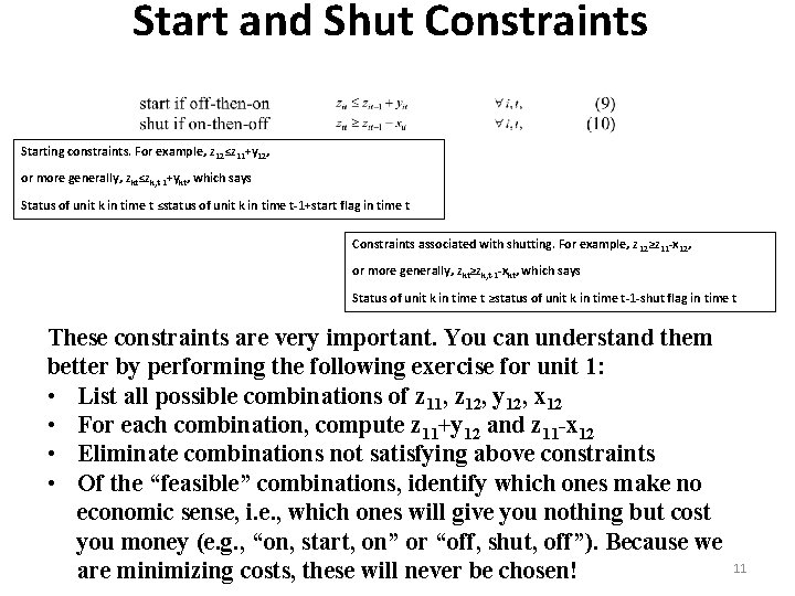
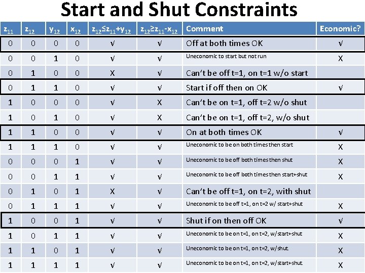
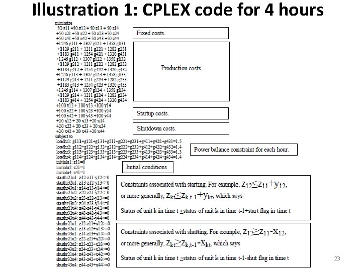
Start and Shut Constraints Starting constraints. For example, z 12≤z 11+y 12, or more generally, zkt≤zk, t-1+ykt, which says Status of unit k in time t ≤status of unit k in time t-1+start flag in time t Constraints associated with shutting. For example, z 12≥z 11 -x 12, or more generally, zkt≥zk, t-1 -xkt, which says Status of unit k in time t ≥status of unit k in time t-1 -shut flag in time t These constraints are very important. You can understand them better by performing the following exercise for unit 1: • List all possible combinations of z 11, z 12, y 12, x 12 • For each combination, compute z 11+y 12 and z 11 -x 12 • Eliminate combinations not satisfying above constraints • Of the “feasible” combinations, identify which ones make no economic sense, i. e. , which ones will give you nothing but cost you money (e. g. , “on, start, on” or “off, shut, off”). Because we are minimizing costs, these will never be chosen! 11

Start and Shut Constraints z 11 z 12 y 12 x 12 z 12≤z 11+y 12 z 12≥z 11 -x 12 Comment Economic? 0 0 √ √ Off at both times OK √ 0 0 1 0 √ √ Uneconomic to start but not run X 0 1 0 0 X √ Can’t be off t=1, on t=1 w/o start 0 1 1 0 √ √ Start if off then on OK 1 0 0 0 √ X Can’t be on t=1, off t=2 w/o shut 1 0 √ X Can’t be on t=1, off t=2, w/o shut 1 1 0 0 √ √ On at both times OK √ 1 1 1 0 √ √ Uneconomic to be on both times then start X 0 0 0 1 √ √ Uneconomic to be off both times then shut X 0 0 1 1 √ √ Uneconomic to be off both times then start+shut X 0 1 X √ Can’t be off t=1, on t=2, with shut 0 1 1 1 √ √ Uneconomic to be off t=1, on t=2 w/ start+shut X 1 0 0 1 √ √ Shut if on then off OK √ 1 0 1 1 √ √ Uneconomic to be on t=1, on t=2, w/start+shut X 1 1 0 1 √ √ Uneconomic to be on t=1, on t=2, w/shut. X 1 1 √ √ Uneconomic to be on t=1, on t=2, w/start+shut. 12 √ X

SCUC Problem (no demand bidding) Subject to Transmission normal constraint Dt is the total demand in period t, SDt is the spinning reserve required in period t, Mx. Inci is max ramprate (MW/period) for increasing gen i output Mx. Deci is max ramprate (MW/period) for decreasing gen i output aij is linearized coefficient relating bus i injection to line k flow Transmisison security constraint, Mx. Flowk is the maximum MW flow on line k is linearized coefficient relating bus i injection to line k flow under contingency j, is the maximum MW flow on line k under contingency j 13 unit i MAXSPi is maximum spinning reserve for

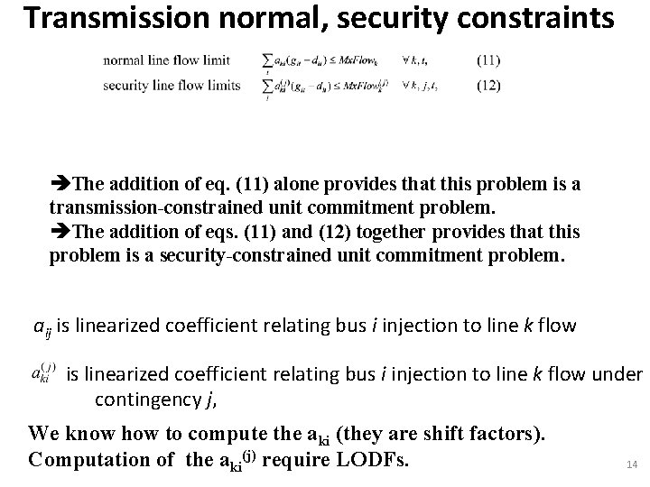
Transmission normal, security constraints The addition of eq. (11) alone provides that this problem is a transmission-constrained unit commitment problem. The addition of eqs. (11) and (12) together provides that this problem is a security-constrained unit commitment problem. aij is linearized coefficient relating bus i injection to line k flow under contingency j, We know how to compute the aki (they are shift factors). Computation of the aki(j) require LODFs. 14

Key Concept Subject to Problem is a function of t. These are intertemporal constraints! In addition to being MIP, the UC problem has two important features. Dynamic: It obtains decisions for a sequence of time periods. Inter-temporal constraints: What happens in one time period affects what happens in another time period. So we may not solve each time period independent of solutions in other time periods. 15

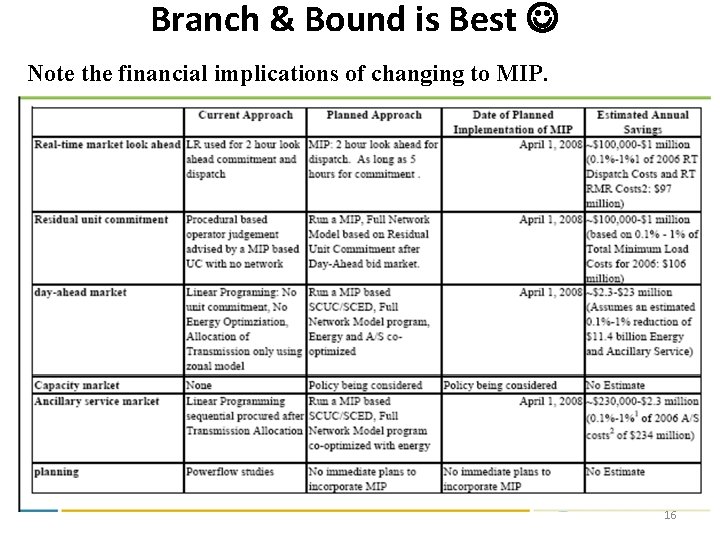
Branch & Bound is Best Note the financial implications of changing to MIP. 16

Some good industry quotes in notes “The most popular algorithms for the solutions of the unit commitment problems are Priority-List schemes [4], Dynamic Programming [5], and Mixed Integer Linear Programming [6]. Among these approaches the MILP technique has achieved significant progress in the recent years [7]. The MILP methodology has been applied to the SCUC formulation to solve this MOW problem. Recent developments in the implementation of MILP-based algorithms and careful attention to the specific problem formulation have made it possible to meet accuracy and performance requirements for solving such large scale problems in a practical competitive energy market environment. ” Q. Zhou, D. Lamb, R. Frowd, E. Ledesma, A. Papalexopoulos, “Minimizing Market Operation Costs Using A Security-Constrained Unit Commitment Approach, ” 2005 IEEE/PES Transmission and Distribution Conference & Exhibition: Asia and Pacific Dalian, China. 17

Some good industry quotes in notes “The LR algorithm was adequate for the original market size, but as the market size increased, PJM desired an approach that had more flexibility in modeling transmission constraints. In addition, PJM has seen an increasing need to model Combined-cycle plant operation more accurately. While these enhancements present a challenge to the LR formulation, the use of a MIP formulation provides much more flexibility. For these reasons, PJM began discussion with its software vendors, in late 2002, concerning the need to develop a production grade MIP-based approach for large-scale unit commitment problems…. ” D. Streiffert, R. Philbrick, and A. Ott, “A Mixed Integer Programming Solution for Market Clearing and Reliability Analysis, ” Power Engineering Society General Meeting, 2005. IEEE 12 -16 June 2005 , pp. 2724 - 2731 Vol. 3. . 18

Some good industry quotes in notes “The Unit Commitment problem is a large-scale non-linear mixed integer programming problem. Integer variables are required for modeling: 1) Generator hourly On/Off-line status, 2) generator Startups/Shutdowns, 3) conditional startup costs (hot, intermediate & cold). Due to the large number of integer variables in this problem, it has long been viewed as an intractable optimization problem. Most existing solution methods make use of simplifying assumptions to reduce the dimensionality of the problem and the number of combinations that need to be evaluated. Examples include priority-based methods, decomposition schemes (LR) and stochastic (genetic) methods. While many of these schemes have worked well in the past, there is an increasing need to solve larger (RTO-size) problems with more complex (e. g. security) constraints, to a greater degree of accuracy. Over the last several years, the number of units being scheduled by RTOs has increased dramatically. PJM started with about 500 units a few years ago, and is now clearing over 1100 each day. MISO cases will be larger still…. ” “The classical MIP implementation utilizes a Branch and Bound scheme. This method attempts to perform an implicit enumeration of all combinations of integer variables to locate the optimal solution. In theory, the MIP is the only method that can make this claim. It can, in fact, solve non-convex problems with multiple local minima. Since the MIP methods utilize multiple Linear Programming (LP) executions, they have benefited from recent advances in both computer hardware and software [6]…” D. Streiffert, R. Philbrick, and A. Ott, “A Mixed Integer Programming Solution for Market Clearing and Reliability 19 Analysis, ” Power Engineering Society General Meeting, 2005. IEEE 12 -16 June 2005 , pp. 2724 - 2731 Vol. 3. .

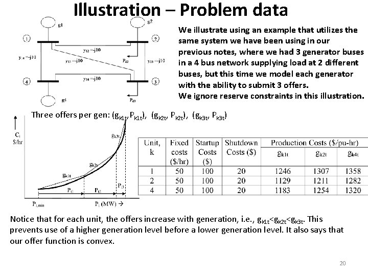
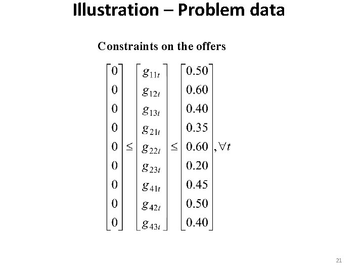
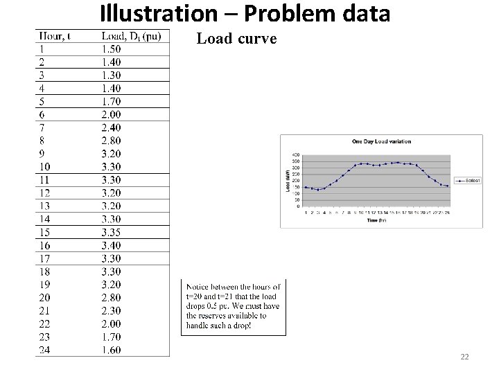
Illustration – Problem data We illustrate using an example that utilizes the same system we have been using in our previous notes, where we had 3 generator buses in a 4 bus network supplying load at 2 different buses, but this time we model each generator with the ability to submit 3 offers. We ignore reserve constraints in this illustration. Three offers per gen: (gk 1 t, Pk 1 t), (gk 2 t, Pk 2 t), (gk 3 t, Pk 3 t) Notice that for each unit, the offers increase with generation, i. e. , g k 1 t<gk 2 t<gk 3 t. This prevents use of a higher generation level before a lower generation level. It also says that our offer function is convex. 20

Illustration – Problem data Constraints on the offers 21

Illustration – Problem data Load curve 22

Illustration 1: CPLEX code for 4 hours 23

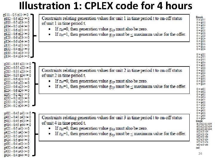
Illustration 1: CPLEX code for 4 hours 24

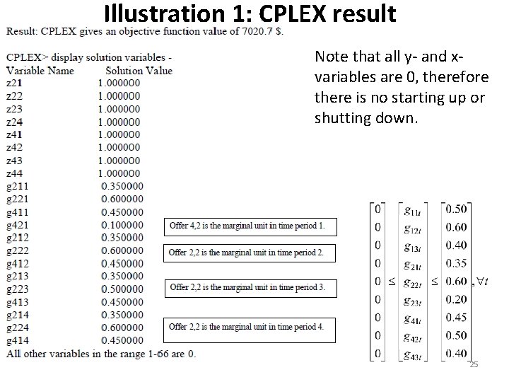
Illustration 1: CPLEX result Note that all y- and xvariables are 0, therefore there is no starting up or shutting down. 25

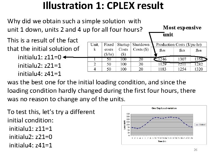
Illustration 1: CPLEX result Why did we obtain such a simple solution with unit 1 down, units 2 and 4 up for all four hours? Most expensive unit This is a result of the fact that the initial solution of initialu 1: z 11=0 initialu 2: z 21=1 initialu 4: z 41=1 was the best one for the initial loading condition, and since the loading condition hardly changed during the first four hours, there was no reason to change any of the units. To test this, let’s try a different initial condition: initialu 1: z 11=1 initialu 2: z 21=0 initialu 4: z 41=1 26

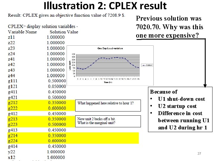
Illustration 2: CPLEX result Previous solution was 7020. 70. Why was this one more expensive? Because of • U 1 shut-down cost • U 2 startup cost • Difference in cost between running U 1 and U 2 during hr 1 27

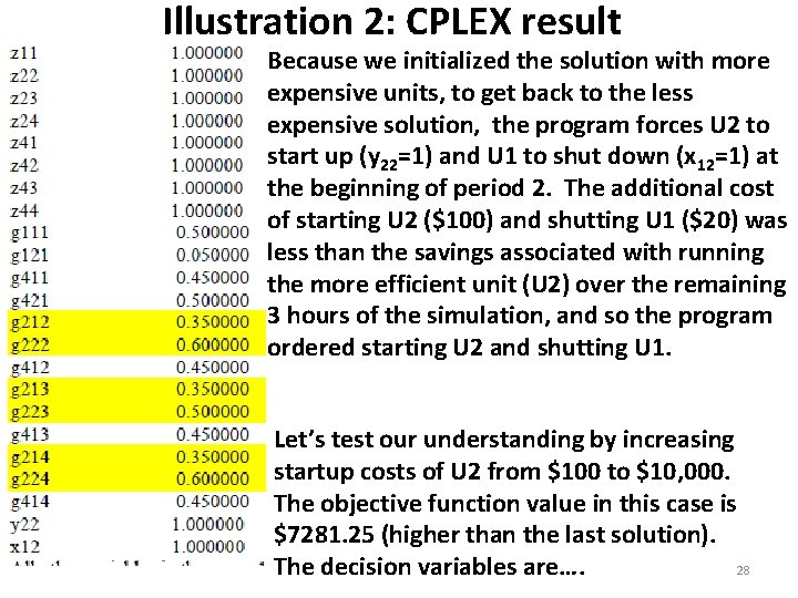
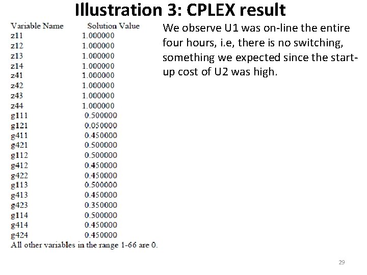
Illustration 2: CPLEX result Because we initialized the solution with more expensive units, to get back to the less expensive solution, the program forces U 2 to start up (y 22=1) and U 1 to shut down (x 12=1) at the beginning of period 2. The additional cost of starting U 2 ($100) and shutting U 1 ($20) was less than the savings associated with running the more efficient unit (U 2) over the remaining 3 hours of the simulation, and so the program ordered starting U 2 and shutting U 1. Let’s test our understanding by increasing startup costs of U 2 from $100 to $10, 000. The objective function value in this case is $7281. 25 (higher than the last solution). 28 The decision variables are….

Illustration 3: CPLEX result We observe U 1 was on-line the entire four hours, i. e, there is no switching, something we expected since the startup cost of U 2 was high. 29

Illustration 4: 24 hours We refrain from showing the data in this case because it is extensive, having 426 variables: 72 z-variables 69 y-variables 69 x-variables 216 g-variables The solution is initialized at initialu 1: z 11=0 initialu 2: z 21=1 initialu 4: z 41=1 which is the most economic solution for the hour 1 loading level. 30

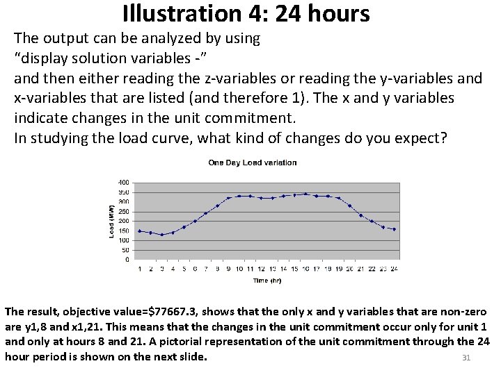
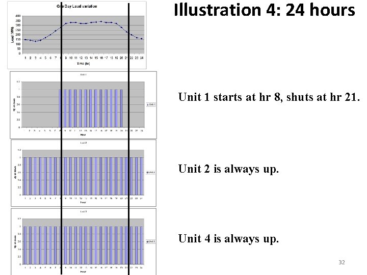
Illustration 4: 24 hours The output can be analyzed by using “display solution variables -” and then either reading the z-variables or reading the y-variables and x-variables that are listed (and therefore 1). The x and y variables indicate changes in the unit commitment. In studying the load curve, what kind of changes do you expect? The result, objective value=$77667. 3, shows that the only x and y variables that are non-zero are y 1, 8 and x 1, 21. This means that the changes in the unit commitment occur only for unit 1 and only at hours 8 and 21. A pictorial representation of the unit commitment through the 24 hour period is shown on the next slide. 31

Illustration 4: 24 hours Unit 1 starts at hr 8, shuts at hr 21. Unit 2 is always up. Unit 4 is always up. 32

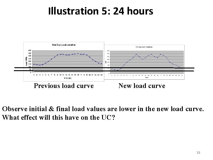
Illustration 5: 24 hours Previous load curve New load curve Observe initial & final load values are lower in the new load curve. What effect will this have on the UC? 33

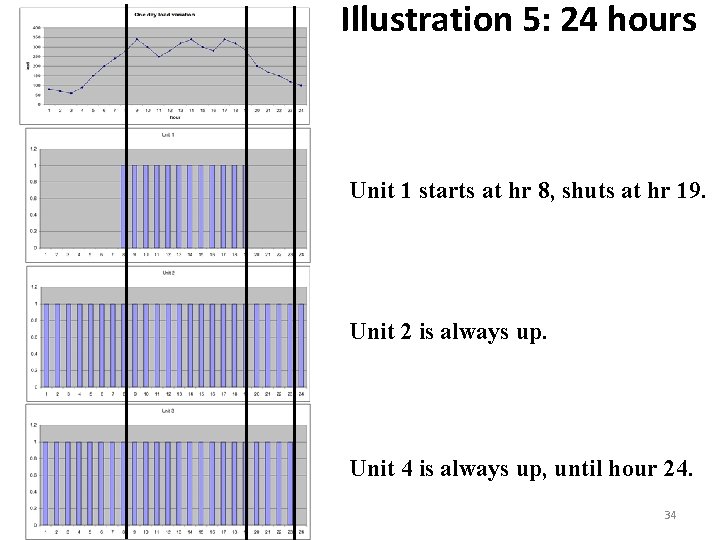
Illustration 5: 24 hours Unit 1 starts at hr 8, shuts at hr 19. Unit 2 is always up. Unit 4 is always up, until hour 24. 34

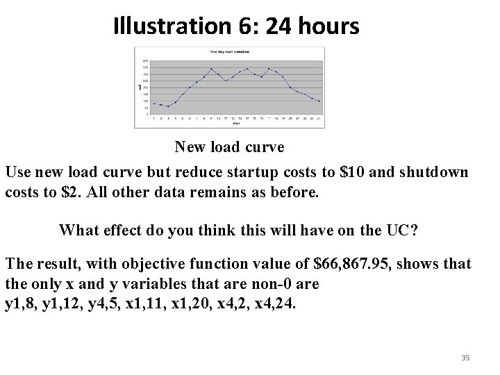
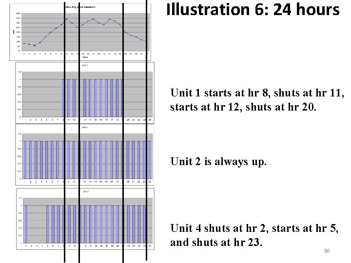
Illustration 6: 24 hours New load curve Use new load curve but reduce startup costs to $10 and shutdown costs to $2. All other data remains as before. What effect do you think this will have on the UC? The result, with objective function value of $66, 867. 95, shows that the only x and y variables that are non-0 are y 1, 8, y 1, 12, y 4, 5, x 1, 11, x 1, 20, x 4, 24. 35

Illustration 6: 24 hours Unit 1 starts at hr 8, shuts at hr 11, starts at hr 12, shuts at hr 20. Unit 2 is always up. Unit 4 shuts at hr 2, starts at hr 5, and shuts at hr 23. 36

An observation What do low start up and shut down costs do to the UC solution? They tend to make UC change more. What do high start up and shut down costs do to the UC solution? They tend to make UC change less. Recall: Inter-temporal constraints: What happens in one time period affects what happens in another time period. So we may not solve each time period independent of solutions in other time periods. Start-up and shut-down costs make the inter-temporal constraints influential. In our problem, if these costs were zero, then the solution we obtain would be the same one we would get 37 if we solved each hour independently.

Another observation Do we obtain the generation dispatch from the UC solution? Yes, these are the gkit variables. Why, then, do we need the SCED? The SCED provides the LMPs, the SCUC does not. After solving any MIP, ask CPLEX for the dual variables using: display solution duals – CPLEX will tell you “Not available for mixed integer problems. ” SCED is solved using LP, which provides dual variables. SCUC is solved using B&B, which cannot provide dual variables. 38

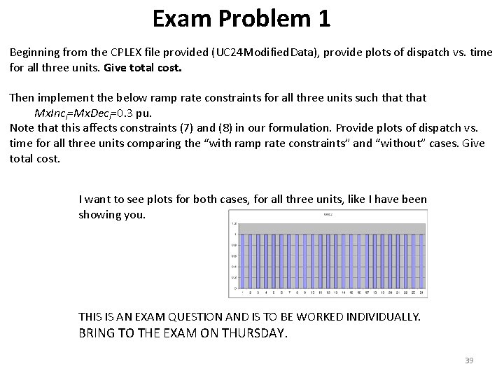
Exam Problem 1 Beginning from the CPLEX file provided (UC 24 Modified. Data), provide plots of dispatch vs. time for all three units. Give total cost. Then implement the below ramp rate constraints for all three units such that Mx. Inci=Mx. Deci=0. 3 pu. Note that this affects constraints (7) and (8) in our formulation. Provide plots of dispatch vs. time for all three units comparing the “with ramp rate constraints” and “without” cases. Give total cost. I want to see plots for both cases, for all three units, like I have been showing you. THIS IS AN EXAM QUESTION AND IS TO BE WORKED INDIVIDUALLY. BRING TO THE EXAM ON THURSDAY. 39

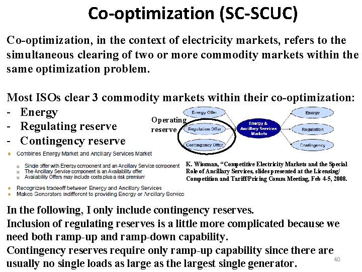
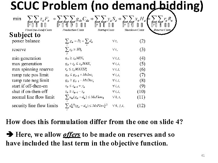
Co-optimization (SC-SCUC) Co-optimization, in the context of electricity markets, refers to the simultaneous clearing of two or more commodity markets within the same optimization problem. Most ISOs clear 3 commodity markets within their co-optimization: - Energy Operating - Regulating reserve - Contingency reserve K. Wissman, “Competitive Electricity Markets and the Special Role of Ancillary Services, slides presented at the Licensing/ Competition and Tariff/Pricing Comm Meeting, Feb 4 -5, 2008. In the following, I only include contingency reserves. Inclusion of regulating reserves is a little more complicated because we need both ramp-up and ramp-down capability. Contingency reserves require only ramp-up capability since there are 40 usually no single loads as large as the largest single generator.

SCUC Problem (no demand bidding) Subject to How does this formulation differ from the on slide 4? Here, we allow offers to be made on reserves and so have included the last term in the objective function. 41

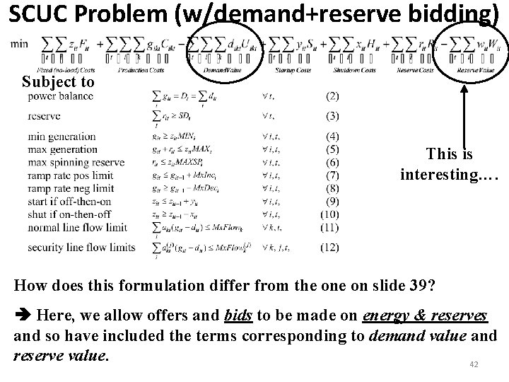
SCUC Problem (w/demand+reserve bidding) Subject to This is interesting…. How does this formulation differ from the on slide 39? Here, we allow offers and bids to be made on energy & reserves and so have included the terms corresponding to demand value and reserve value. 42

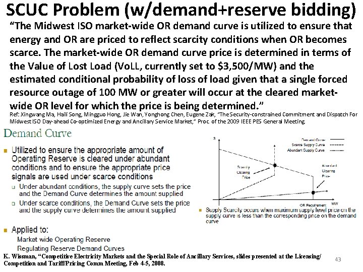
SCUC Problem (w/demand+reserve bidding) “The Midwest ISO market-wide OR demand curve is utilized to ensure that energy and OR are priced to reflect scarcity conditions when OR becomes scarce. The market-wide OR demand curve price is determined in terms of the Value of Lost Load (Vo. LL, currently set to $3, 500/MW) and the estimated conditional probability of loss of load given that a single forced resource outage of 100 MW or greater will occur at the cleared marketwide OR level for which the price is being determined. ” Ref: Xingwang Ma, Haili Song, Mingguo Hong, Jie Wan, Yonghong Chen, Eugene Zak, “The Security-constrained Commitment and Dispatch For Midwest ISO Day-ahead Co-optimized Energy and Ancillary Service Market, ” Proc. of the 2009 IEEE PES General Meeting. K. Wissman, “Competitive Electricity Markets and the Special Role of Ancillary Services, slides presented at the Licensing/ Competition and Tariff/Pricing Comm Meeting, Feb 4 -5, 2008. 43