EEEcon 458 LPOPF J Mc Calley 1 LPOPF

EE/Econ 458 LPOPF J. Mc. Calley 1

LPOPF The linear program optimal power flow is functionally equivalent to the SCED (but not to the SC-SCED). The main difference is that LPOPF uses DC power flow equations whereas SCED uses linear sensitivities (generation shift factors). Please read below papers posted to website for full description of SC-SCUC and SC-SCED. Ref: Xingwang Ma, Haili Song, Mingguo Hong, Jie Wan, Yonghong Chen, Eugene Zak, “The Security-constrained Commitment and Dispatch For Midwest ISO Day-ahead Co-optimized Energy and Ancillary Service Market, ” Proc. of the 2009 IEEE PES General Meeting. Ref: Xingwang Ma, Yonghong Chen, Jie Wan, “Midwest ISO Co-optimization Based Real-time Dispatch and Pricing of Energy and Ancillary Services, ” Proc. of the 2009 IEEE PES General Meeting. 2

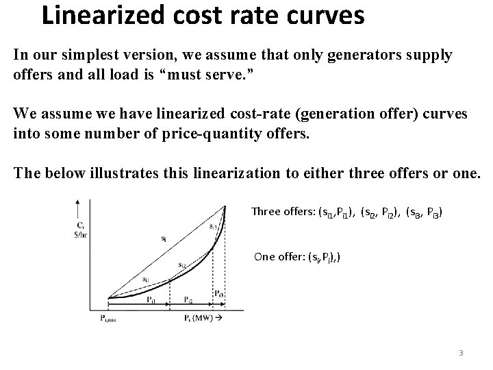
Linearized cost rate curves In our simplest version, we assume that only generators supply offers and all load is “must serve. ” We assume we have linearized cost-rate (generation offer) curves into some number of price-quantity offers. The below illustrates this linearization to either three offers or one. Three offers: (si 1, Pi 1), (si 2, Pi 2), (si 3, Pi 3) One offer: (si, Pi), ) 3

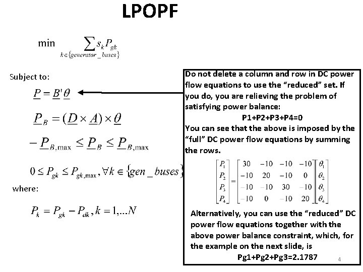
LPOPF Subject to: Do not delete a column and row in DC power flow equations to use the “reduced” set. If you do, you are relieving the problem of satisfying power balance: P 1+P 2+P 3+P 4=0 You can see that the above is imposed by the “full” DC power flow equations by summing the rows. where: Alternatively, you can use the “reduced” DC power flow equations together with the above power balance constraint, which, for the example on the next slide, is Pg 1+Pg 2+Pg 3=2. 1787 4

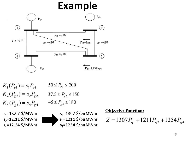
Example , s 1=13. 07 $/MWhr s 2=12. 11 $/MWhr s 4=12. 54 $/MWhr s 1=1307 $/pu. MWhr s 2=1211 $/pu. MWhr s 4=1254 $/pu. MWhr Objective function: 5

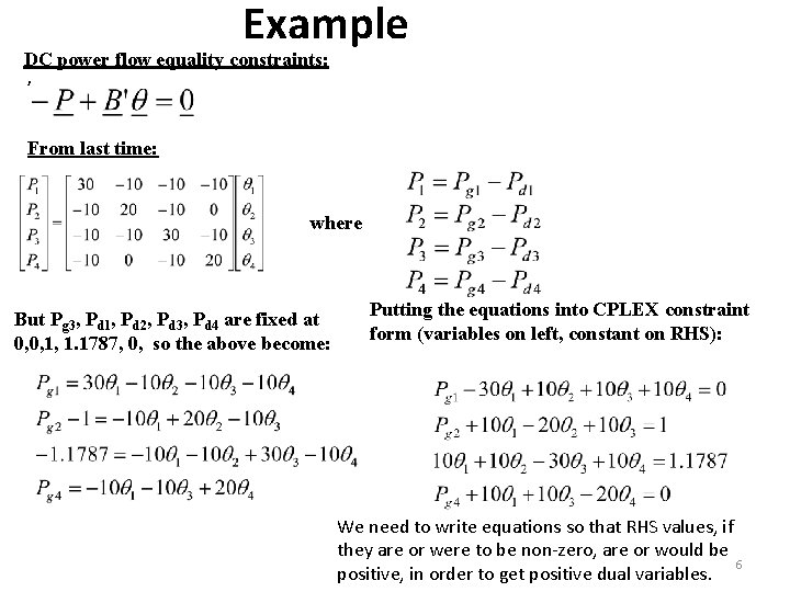
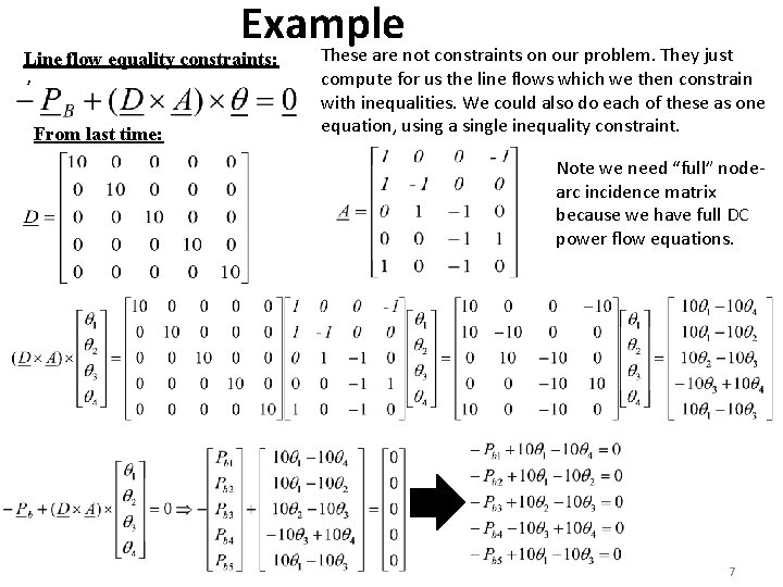
Example DC power flow equality constraints: , From last time: where But Pg 3, Pd 1, Pd 2, Pd 3, Pd 4 are fixed at 0, 0, 1, 1. 1787, 0, so the above become: Putting the equations into CPLEX constraint form (variables on left, constant on RHS): We need to write equations so that RHS values, if they are or were to be non-zero, are or would be 6 positive, in order to get positive dual variables.

Example These are not constraints on our problem. They just Line flow equality constraints: , From last time: compute for us the line flows which we then constrain with inequalities. We could also do each of these as one equation, using a single inequality constraint. Note we need “full” nodearc incidence matrix because we have full DC power flow equations. 7

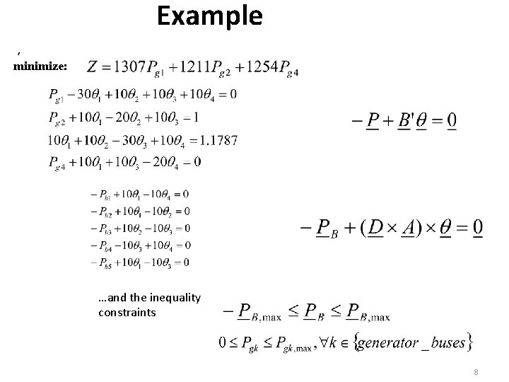
Example , minimize: …and the inequality constraints 8

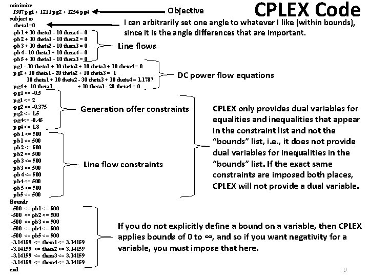
CPLEX Code minimize 1307 pg 1 + 1211 pg 2 + 1254 pg 4 subject to I can arbitrarily set one angle to whatever I like (within theta 1=0 -pb 1 + 10 theta 1 - 10 theta 4 = 0 since it is the angle differences that are important. -pb 2 + 10 theta 1 - 10 theta 2 = 0 -pb 3 + 10 theta 2 - 10 theta 3 = 0 -pb 4 - 10 theta 3 + 10 theta 4 = 0 -pb 5 + 10 theta 1 - 10 theta 3 = 0 pg 1 - 30 theta 1 + 10 theta 2 + 10 theta 3 + 10 theta 4 = 0 pg 2 + 10 theta 1 - 20 theta 2 + 10 theta 3 = 1 10 theta 1 + 10 theta 2 - 30 theta 3 + 10 theta 4 = 1. 1787 pg 4 + 10 theta 1 + 10 theta 3 - 20 theta 4 = 0 -pg 1 <= -0. 5 pg 1 <= 2 -pg 2 <= -0. 375 pg 2 <= 1. 5 -pg 4<= -0. 45 pg 4 <= 1. 8 -pb 1 <= 500 -pb 2 <= 500 -pb 3 <= 500 -pb 4 <= 500 -pb 5 <= 500 Bounds -500 <= pb 1 <= 500 -500 <= pb 2 <= 500 -500 <= pb 3 <= 500 -500 <= pb 4 <= 500 -500 <= pb 5 <= 500 -3. 14159 <= theta 1 <= 3. 14159 -3. 14159 <= theta 2 <= 3. 14159 -3. 14159 <= theta 3 <= 3. 14159 -3. 14159 <= theta 4 <= 3. 14159 end Objective bounds), Line flows DC power flow equations Generation offer constraints Line flow constraints CPLEX only provides dual variables for equalities and inequalities that appear in the constraint list and not the “bounds” list, i. e. , it does not provide dual variables for inequalities in the “bounds” list. If the exact same constraints are imposed both places, CPLEX will not provide a dual variable. If you do not explicitly define a bound on a variable, then CPLEX applies bounds of 0 to ∞, and so if you want negativity for a variable, you must impose that here. 9

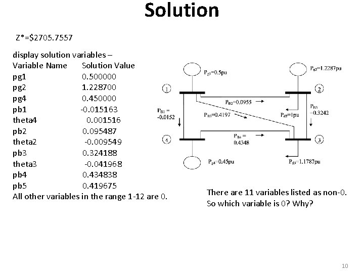
Solution Z*=$2705. 7557 display solution variables – Variable Name Solution Value pg 1 0. 500000 pg 2 1. 228700 pg 4 0. 450000 pb 1 -0. 015163 theta 4 0. 001516 pb 2 0. 095487 theta 2 -0. 009549 pb 3 0. 324188 theta 3 -0. 041968 pb 4 0. 434838 pb 5 0. 419675 All other variables in the range 1 -12 are 0. There are 11 variables listed as non-0. So which variable is 0? Why? 10

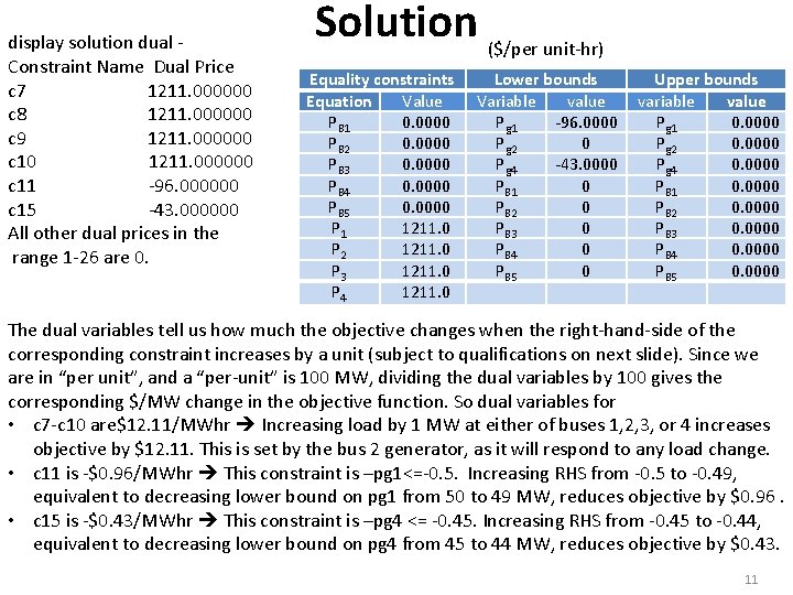
display solution dual Constraint Name Dual Price c 7 1211. 000000 c 8 1211. 000000 c 9 1211. 000000 c 10 1211. 000000 c 11 -96. 000000 c 15 -43. 000000 All other dual prices in the range 1 -26 are 0. Solution ($/per unit-hr) Equality constraints Equation Value PB 1 0. 0000 PB 2 0. 0000 PB 3 0. 0000 PB 4 0. 0000 PB 5 0. 0000 P 1 1211. 0 P 2 1211. 0 P 3 1211. 0 P 4 1211. 0 Lower bounds Variable value Pg 1 -96. 0000 Pg 2 0 Pg 4 -43. 0000 PB 1 0 PB 2 0 PB 3 0 PB 4 0 PB 5 0 Upper bounds variable value Pg 1 0. 0000 Pg 2 0. 0000 Pg 4 0. 0000 PB 1 0. 0000 PB 2 0. 0000 PB 3 0. 0000 PB 4 0. 0000 PB 5 0. 0000 The dual variables tell us how much the objective changes when the right-hand-side of the corresponding constraint increases by a unit (subject to qualifications on next slide). Since we are in “per unit”, and a “per-unit” is 100 MW, dividing the dual variables by 100 gives the corresponding $/MW change in the objective function. So dual variables for • c 7 -c 10 are$12. 11/MWhr Increasing load by 1 MW at either of buses 1, 2, 3, or 4 increases objective by $12. 11. This is set by the bus 2 generator, as it will respond to any load change. • c 11 is -$0. 96/MWhr This constraint is –pg 1<=-0. 5. Increasing RHS from -0. 5 to -0. 49, equivalent to decreasing lower bound on pg 1 from 50 to 49 MW, reduces objective by $0. 96. • c 15 is -$0. 43/MWhr This constraint is –pg 4 <= -0. 45. Increasing RHS from -0. 45 to -0. 44, equivalent to decreasing lower bound on pg 4 from 45 to 44 MW, reduces objective by $0. 43. 11

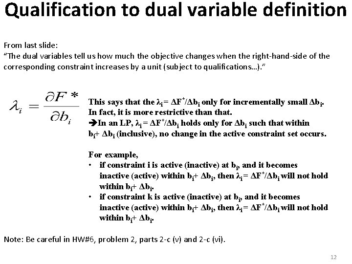
Qualification to dual variable definition From last slide: “The dual variables tell us how much the objective changes when the right-hand-side of the corresponding constraint increases by a unit (subject to qualifications…). ” This says that the λi = ΔF*/Δbi only for incrementally small Δbi. In fact, it is more restrictive than that. In an LP, λi = ΔF*/Δbi holds only for Δbi such that within bi+ Δbi (inclusive), no change in the active constraint set occurs. For example, • if constraint i is active (inactive) at bi, and it becomes inactive (active) within bi+ Δbi, then λi = ΔF*/Δbi will not hold within bi+ Δbi. • if constraint k is active (inactive) at bi, and it becomes inactive (active) within bi+ Δbi, then λi = ΔF*/Δbi will not hold within bi+ Δbi. Note: Be careful in HW#6, problem 2, parts 2 -c (v) and 2 -c (vi). 12

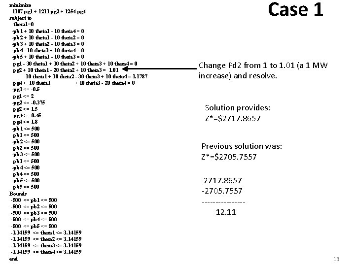
minimize 1307 pg 1 + 1211 pg 2 + 1254 pg 4 subject to theta 1=0 -pb 1 + 10 theta 1 - 10 theta 4 = 0 -pb 2 + 10 theta 1 - 10 theta 2 = 0 -pb 3 + 10 theta 2 - 10 theta 3 = 0 -pb 4 - 10 theta 3 + 10 theta 4 = 0 -pb 5 + 10 theta 1 - 10 theta 3 = 0 pg 1 - 30 theta 1 + 10 theta 2 + 10 theta 3 + 10 theta 4 = 0 pg 2 + 10 theta 1 - 20 theta 2 + 10 theta 3 = 1. 01 10 theta 1 + 10 theta 2 - 30 theta 3 + 10 theta 4 = 1. 1787 pg 4 + 10 theta 1 + 10 theta 3 - 20 theta 4 = 0 -pg 1 <= -0. 5 pg 1 <= 2 -pg 2 <= -0. 375 pg 2 <= 1. 5 -pg 4<= -0. 45 pg 4 <= 1. 8 -pb 1 <= 500 -pb 2 <= 500 -pb 3 <= 500 -pb 4 <= 500 -pb 5 <= 500 Bounds -500 <= pb 1 <= 500 -500 <= pb 2 <= 500 -500 <= pb 3 <= 500 -500 <= pb 4 <= 500 -500 <= pb 5 <= 500 -3. 14159 <= theta 1 <= 3. 14159 -3. 14159 <= theta 2 <= 3. 14159 -3. 14159 <= theta 3 <= 3. 14159 -3. 14159 <= theta 4 <= 3. 14159 end Case 1 Change Pd 2 from 1 to 1. 01 (a 1 MW increase) and resolve. Solution provides: Z*=$2717. 8657 Previous solution was: Z*=$2705. 7557 2717. 8657 -2705. 7557 -------- 12. 11 13

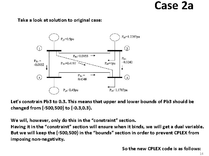
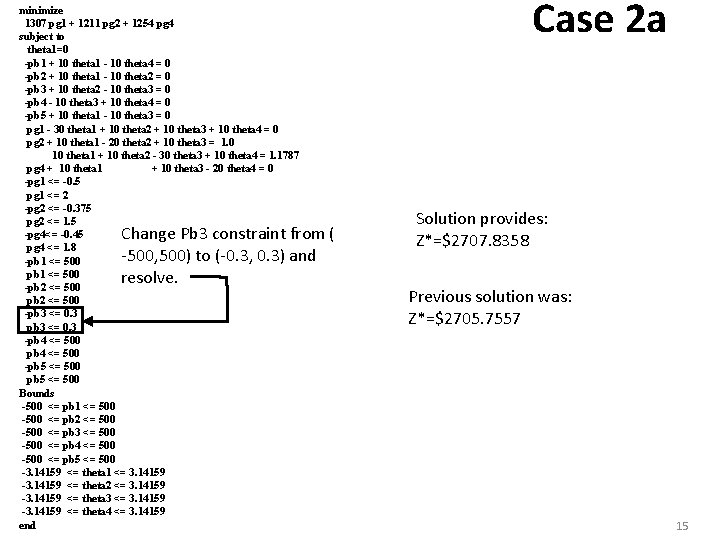
Case 2 a Take a look at solution to original case: Let’s constrain Pb 3 to 0. 3. This means that upper and lower bounds of Pb 3 should be changed from (-500, 500) to (-0. 3, 0. 3). We will, however, only do this in the “constraint” section. Having it in the “constraint” section will ensure when it binds, we will get a dual variable. But we will keep the (-500, 500) in the “bounds” section in order to prevent CPLEX from imposing non-negativity. So the new CPLEX code is as follows: 14

minimize 1307 pg 1 + 1211 pg 2 + 1254 pg 4 subject to theta 1=0 -pb 1 + 10 theta 1 - 10 theta 4 = 0 -pb 2 + 10 theta 1 - 10 theta 2 = 0 -pb 3 + 10 theta 2 - 10 theta 3 = 0 -pb 4 - 10 theta 3 + 10 theta 4 = 0 -pb 5 + 10 theta 1 - 10 theta 3 = 0 pg 1 - 30 theta 1 + 10 theta 2 + 10 theta 3 + 10 theta 4 = 0 pg 2 + 10 theta 1 - 20 theta 2 + 10 theta 3 = 1. 0 10 theta 1 + 10 theta 2 - 30 theta 3 + 10 theta 4 = 1. 1787 pg 4 + 10 theta 1 + 10 theta 3 - 20 theta 4 = 0 -pg 1 <= -0. 5 pg 1 <= 2 -pg 2 <= -0. 375 pg 2 <= 1. 5 -pg 4<= -0. 45 pg 4 <= 1. 8 -pb 1 <= 500 -pb 2 <= 500 -pb 3 <= 0. 3 -pb 4 <= 500 -pb 5 <= 500 Bounds -500 <= pb 1 <= 500 -500 <= pb 2 <= 500 -500 <= pb 3 <= 500 -500 <= pb 4 <= 500 -500 <= pb 5 <= 500 -3. 14159 <= theta 1 <= 3. 14159 -3. 14159 <= theta 2 <= 3. 14159 -3. 14159 <= theta 3 <= 3. 14159 -3. 14159 <= theta 4 <= 3. 14159 end Change Pb 3 constraint from ( -500, 500) to (-0. 3, 0. 3) and resolve. Case 2 a Solution provides: Z*=$2707. 8358 Previous solution was: Z*=$2705. 7557 15

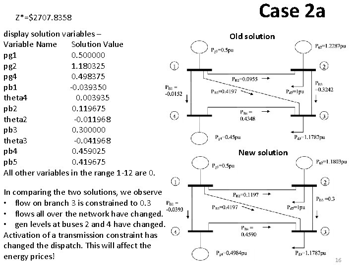
Z*=$2707. 8358 display solution variables – Variable Name Solution Value pg 1 0. 500000 pg 2 1. 180325 pg 4 0. 498375 pb 1 -0. 039350 theta 4 0. 003935 pb 2 0. 119675 theta 2 -0. 011968 pb 3 0. 300000 theta 3 -0. 041968 pb 4 0. 459025 pb 5 0. 419675 All other variables in the range 1 -12 are 0. In comparing the two solutions, we observe • flow on branch 3 is constrained to 0. 3 • flows all over the network have changed. • gen levels at buses 2 and 4 have changed. Activation of a transmission constraint has changed the dispatch. This will affect the energy prices! Case 2 a Old solution New solution 16

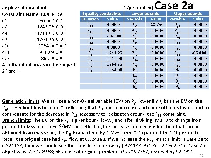
Case 2 a display solution dual ($/per unit-hr) Equality constraints Lower bounds Constraint Name Dual Price Equation Value Variable value c 4 -86. 000000 PB 1 0. 0000 Pg 1 -63. 750 c 7 1243. 250000 PB 2 0. 0000 Pg 2 0. 0000 c 8 1211. 000000 PB 3 -86. 000 Pg 4 0. 0000 c 9 1264. 750000 PB 4 0. 0000 PB 1 0. 0000 c 10 1254. 000000 PB 5 0. 0000 PB 2 0. 0000 c 11 -63. 750000 P 1 1243. 25 PB 3 0. 0000 P 2 1211. 00 PB 4 0. 0000 c 22 -86. 000000 P 3 1264. 75 PB 5 0. 0000 All other dual prices in the range 1 P 4 1254. 00 θ 1 0. 0000 26 are 0. θ 2 θ 3 θ 4 0. 0000 Upper bounds variable value Pg 1 0. 0000 Pg 2 0. 0000 Pg 4 0. 0000 PB 1 0. 0000 PB 2 0. 0000 PB 3 -86. 000 PB 4 0. 0000 PB 5 0. 0000 θ 1 0. 0000 θ 2 0. 0000 θ 3 0. 0000 θ 4 0. 0000 Generation limits: We still see a non-0 dual variable (DV) on Pg 1 lower limit, but the DV on the Pg 4 lower limit has become 0, reflecting that Pg 4 had to increase and come off of its lower limit to compensate for the decrease in Pg 2 necessary to redispatch around the PB 3 constraint. Branch limits: The DV on the PB 3 upper bound is -86, and after dividing by 100 to change from per-unit to MW, it is -0. 86 $/MW-hr, reflecting the increase in objective function that can be obtained from increasing the PB 3 branch limit by 1 MW (from 0. 30 per-unit to 0. 31 per-unit). Recall the original case had PB 3 flow at 0. 324188. If we increase the PB 3 branch limit in Case 2 a to 0. 324188, then we should see the objective increase by (. 324188 -. 3)*-86=-2. 0802. Our Case 2 a objective is $2707. 8358; objective of original problem is $2705. 7557, reduced by $2. 0801. 17

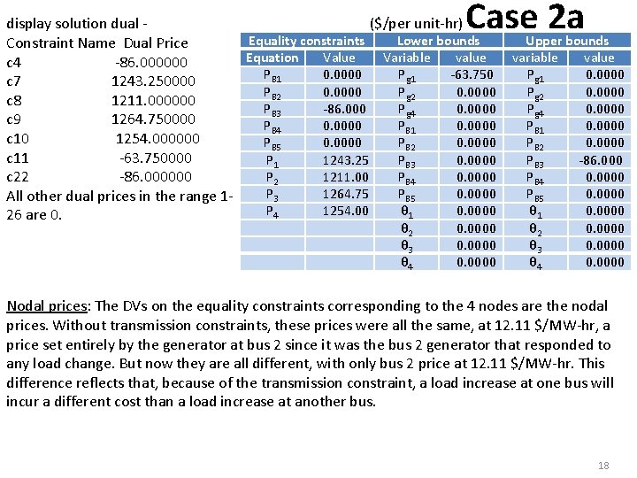
Case 2 a display solution dual ($/per unit-hr) Equality constraints Lower bounds Constraint Name Dual Price Equation Value Variable value c 4 -86. 000000 PB 1 0. 0000 Pg 1 -63. 750 c 7 1243. 250000 PB 2 0. 0000 Pg 2 0. 0000 c 8 1211. 000000 PB 3 -86. 000 Pg 4 0. 0000 c 9 1264. 750000 PB 4 0. 0000 PB 1 0. 0000 c 10 1254. 000000 PB 5 0. 0000 PB 2 0. 0000 c 11 -63. 750000 P 1 1243. 25 PB 3 0. 0000 P 2 1211. 00 PB 4 0. 0000 c 22 -86. 000000 P 3 1264. 75 PB 5 0. 0000 All other dual prices in the range 1 P 4 1254. 00 θ 1 0. 0000 26 are 0. θ 2 θ 3 θ 4 0. 0000 Upper bounds variable value Pg 1 0. 0000 Pg 2 0. 0000 Pg 4 0. 0000 PB 1 0. 0000 PB 2 0. 0000 PB 3 -86. 000 PB 4 0. 0000 PB 5 0. 0000 θ 1 0. 0000 θ 2 0. 0000 θ 3 0. 0000 θ 4 0. 0000 Nodal prices: The DVs on the equality constraints corresponding to the 4 nodes are the nodal prices. Without transmission constraints, these prices were all the same, at 12. 11 $/MW-hr, a price set entirely by the generator at bus 2 since it was the bus 2 generator that responded to any load change. But now they are all different, with only bus 2 price at 12. 11 $/MW-hr. This difference reflects that, because of the transmission constraint, a load increase at one bus will incur a different cost than a load increase at another bus. 18

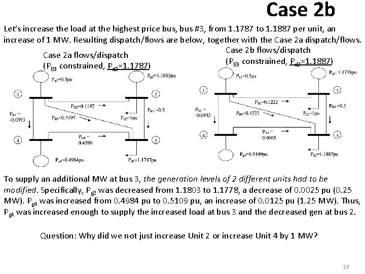
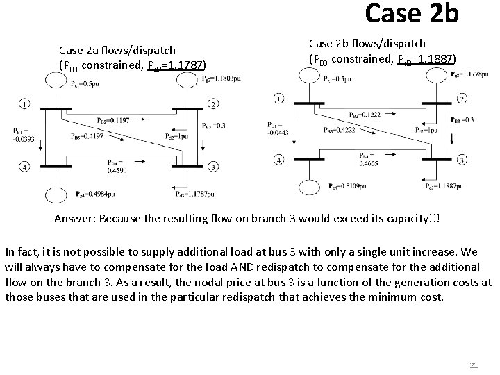
Case 2 b Let’s increase the load at the highest price bus, bus #3, from 1. 1787 to 1. 1887 per unit, an increase of 1 MW. Resulting dispatch/flows are below, together with the Case 2 a dispatch/flows. Case 2 b flows/dispatch Case 2 a flows/dispatch (PB 3 constrained, Pd 2=1. 1887) (PB 3 constrained, Pd 2=1. 1787) To supply an additional MW at bus 3, the generation levels of 2 different units had to be modified. Specifically, Pg 2 was decreased from 1. 1803 to 1. 1778, a decrease of 0. 0025 pu (0. 25 MW). Pg 4 was increased from 0. 4984 pu to 0. 5109 pu, an increase of 0. 0125 pu (1. 25 MW). Thus, Pg 4 was increased enough to supply the increased load at bus 3 and the decreased gen at bus 2. Question: Why did we not just increase Unit 2 or increase Unit 4 by 1 MW? 19

Case 2 b Case 2 a flows/dispatch (PB 3 constrained, Pd 2=1. 1787) Case 2 b flows/dispatch (PB 3 constrained, Pd 2=1. 1887) Answer: Because the resulting flow on branch 3 would exceed its capacity!!! In fact, it is not possible to supply additional load at bus 3 with only a single unit increase. We will always have to compensate for the load AND redispatch to compensate for the additional flow on the branch 3. As a result, the nodal price at bus 3 is a function of the generation costs at those buses that are used in the particular redispatch that achieves the minimum cost. 20

Case 2 b Case 2 a flows/dispatch (PB 3 constrained, Pd 2=1. 1787) Case 2 b flows/dispatch (PB 3 constrained, Pd 2=1. 1887) Answer: Because the resulting flow on branch 3 would exceed its capacity!!! In fact, it is not possible to supply additional load at bus 3 with only a single unit increase. We will always have to compensate for the load AND redispatch to compensate for the additional flow on the branch 3. As a result, the nodal price at bus 3 is a function of the generation costs at those buses that are used in the particular redispatch that achieves the minimum cost. 21

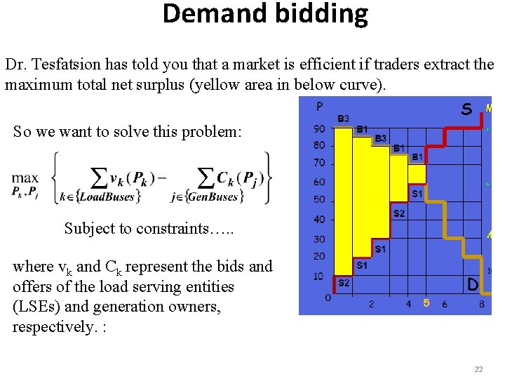
Demand bidding Dr. Tesfatsion has told you that a market is efficient if traders extract the maximum total net surplus (yellow area in below curve). So we want to solve this problem: Subject to constraints…. . where vk and Ck represent the bids and offers of the load serving entities (LSEs) and generation owners, respectively. : 22

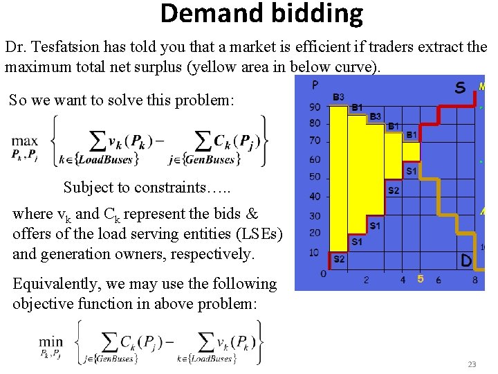
Demand bidding Dr. Tesfatsion has told you that a market is efficient if traders extract the maximum total net surplus (yellow area in below curve). So we want to solve this problem: Subject to constraints…. . where vk and Ck represent the bids & offers of the load serving entities (LSEs) and generation owners, respectively. Equivalently, we may use the following objective function in above problem: 23

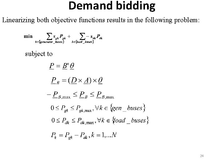
Demand bidding Linearizing both objective functions results in the following problem: subject to 24

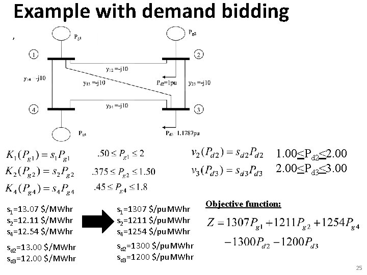
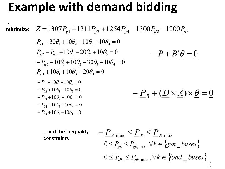
Example with demand bidding , 1. 00<Pd 2<2. 00<Pd 3<3. 00 s 1=13. 07 $/MWhr s 2=12. 11 $/MWhr s 4=12. 54 $/MWhr s 1=1307 $/pu. MWhr s 2=1211 $/pu. MWhr s 4=1254 $/pu. MWhr sd 2=13. 00 $/MWhr sd 3=12. 00 $/MWhr sd 2=1300 $/pu. MWhr sd 3=1200 $/pu. MWhr Objective function: 25

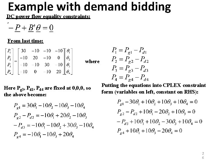
Example with demand bidding DC power flow equality constraints: , From last time: where Here Pg 3, Pd 1, Pd 4 are fixed at 0, 0, 0, so the above become: Putting the equations into CPLEX constraint form (variables on left, constant on RHS): 2 6

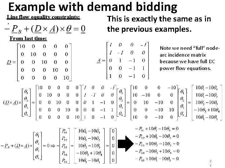
Example with demand bidding Line flow equality constraints: , This is exactly the same as in the previous examples. From last time: Note we need “full” nodearc incidence matrix because we have full DC power flow equations. 2 7

Example with demand bidding , minimize: …and the inequality constraints 2 8

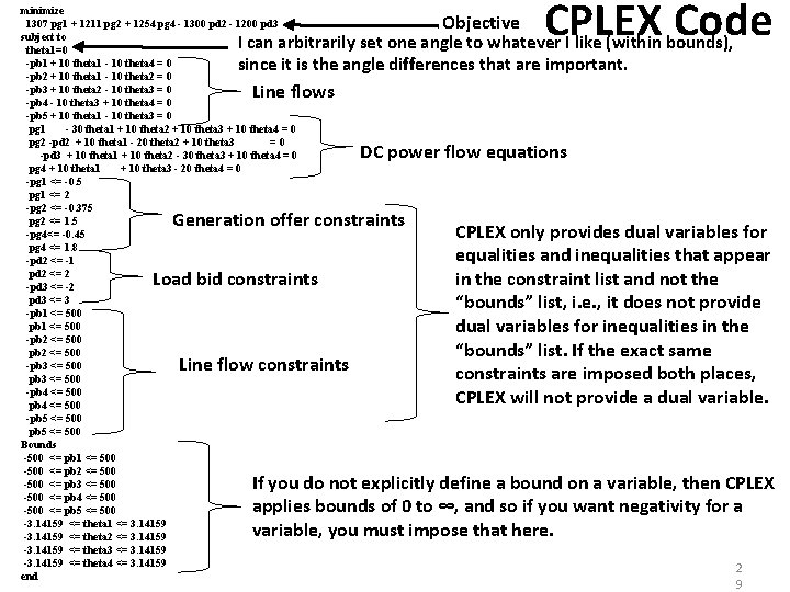
minimize 1307 pg 1 + 1211 pg 2 + 1254 pg 4 - 1300 pd 2 - 1200 pd 3 subject to theta 1=0 -pb 1 + 10 theta 1 - 10 theta 4 = 0 -pb 2 + 10 theta 1 - 10 theta 2 = 0 -pb 3 + 10 theta 2 - 10 theta 3 = 0 -pb 4 - 10 theta 3 + 10 theta 4 = 0 -pb 5 + 10 theta 1 - 10 theta 3 = 0 pg 1 - 30 theta 1 + 10 theta 2 + 10 theta 3 + 10 theta 4 = 0 pg 2 -pd 2 + 10 theta 1 - 20 theta 2 + 10 theta 3 =0 -pd 3 + 10 theta 1 + 10 theta 2 - 30 theta 3 + 10 theta 4 = 0 pg 4 + 10 theta 1 + 10 theta 3 - 20 theta 4 = 0 -pg 1 <= -0. 5 pg 1 <= 2 -pg 2 <= -0. 375 pg 2 <= 1. 5 -pg 4<= -0. 45 pg 4 <= 1. 8 -pd 2 <= -1 pd 2 <= 2 -pd 3 <= -2 pd 3 <= 3 -pb 1 <= 500 -pb 2 <= 500 -pb 3 <= 500 -pb 4 <= 500 -pb 5 <= 500 Bounds -500 <= pb 1 <= 500 -500 <= pb 2 <= 500 -500 <= pb 3 <= 500 -500 <= pb 4 <= 500 -500 <= pb 5 <= 500 -3. 14159 <= theta 1 <= 3. 14159 -3. 14159 <= theta 2 <= 3. 14159 -3. 14159 <= theta 3 <= 3. 14159 -3. 14159 <= theta 4 <= 3. 14159 end Objective CPLEX Code I can arbitrarily set one angle to whatever I like (within bounds), since it is the angle differences that are important. Line flows DC power flow equations Generation offer constraints Load bid constraints Line flow constraints CPLEX only provides dual variables for equalities and inequalities that appear in the constraint list and not the “bounds” list, i. e. , it does not provide dual variables for inequalities in the “bounds” list. If the exact same constraints are imposed both places, CPLEX will not provide a dual variable. If you do not explicitly define a bound on a variable, then CPLEX applies bounds of 0 to ∞, and so if you want negativity for a variable, you must impose that here. 2 9

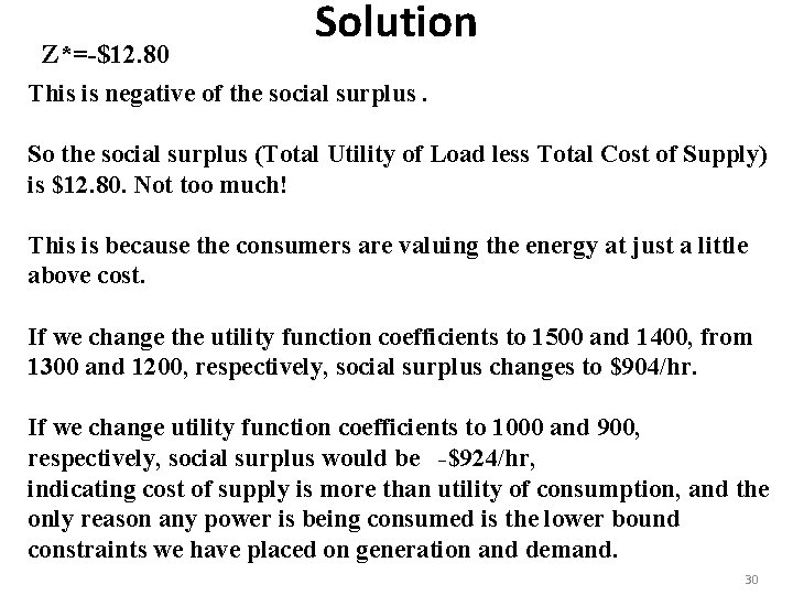
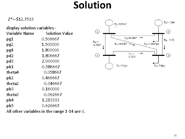
Solution Z*=-$12. 80 This is negative of the social surplus. So the social surplus (Total Utility of Load less Total Cost of Supply) is $12. 80. Not too much! This is because the consumers are valuing the energy at just a little above cost. If we change the utility function coefficients to 1500 and 1400, from 1300 and 1200, respectively, social surplus changes to $904/hr. If we change utility function coefficients to 1000 and 900, respectively, social surplus would be -$924/hr, indicating cost of supply is more than utility of consumption, and the only reason any power is being consumed is the lower bound constraints we have placed on generation and demand. 30

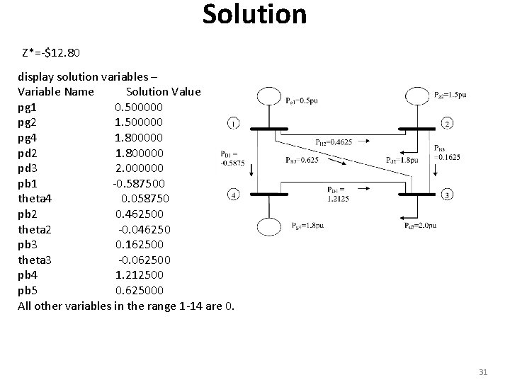
Solution Z*=-$12. 80 display solution variables – Variable Name Solution Value pg 1 0. 500000 pg 2 1. 500000 pg 4 1. 800000 pd 2 1. 800000 pd 3 2. 000000 pb 1 -0. 587500 theta 4 0. 058750 pb 2 0. 462500 theta 2 -0. 046250 pb 3 0. 162500 theta 3 -0. 062500 pb 4 1. 212500 pb 5 0. 625000 All other variables in the range 1 -14 are 0. 31

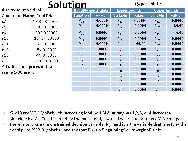
Solution display solution dual Constraint Name Dual Price c 7 1300. 000000 c 8 1300. 000000 c 9 1300. 000000 c 10 1300. 000000 c 11 -7. 000000 c 14 -89. 000000 c 16 -46. 000000 c 19 -100. 000000 All other dual prices in the range 1 -30 are 0. ($/per unit-hr) Equality constraints Equation Value PB 1 -0. 0000 PB 2 -0. 0000 PB 3 PB 4 PB 5 P 1 P 2 P 3 P 4 0. 0000 -0. 0000 1300. 0 Lower bounds Variable value Pg 1 -7. 0000 Pg 2 0. 0000 Pg 4 Pd 2 Pd 3 PB 1 PB 2 PB 3 PB 4 PB 5 θ 1 θ 2 θ 3 θ 4 0. 0000 -100. 0000 0. 0000 Upper bounds variable value Pg 1 0. 0000 Pg 2 -89. 00 Pg 4 Pd 2 PB 1 PB 2 PB 3 PB 4 PB 5 θ 1 θ 2 θ 3 θ 4 -46. 00 0. 0000 0. 0000 • c 7 -c 10 are$13. 00/MWhr Increasing load by 1 MW at any bus 1, 2, 3, or 4 increases objective by $13. 00. This is set by the bus 2 load, Pd 2, as it will respond to any MW change. • There is only one unconstrained decision variable, Pd 2, and it is the variable that is setting the nodal price ($13. 00/MWhr). We say that Pd 2 is a “regulating” or “marginal” unit. 32

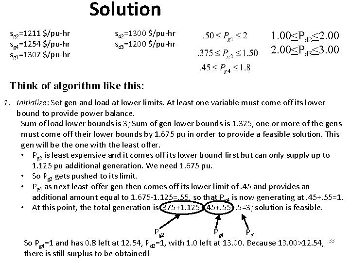
Solution sg 2=1211 $/pu-hr sg 4=1254 $/pu-hr sg 1=1307 $/pu-hr sd 2=1300 $/pu-hr sd 3=1200 $/pu-hr 1. 00<Pd 2<2. 00<Pd 3<3. 00 Think of algorithm like this: 1. Initialize: Set gen and load at lower limits. At least one variable must come off its lower bound to provide power balance. Sum of load lower bounds is 3; Sum of gen lower bounds is 1. 325, one or more of the gens must come off their lower bounds by 1. 675 pu in order to provide a feasible solution. This gen will be the one with the least offer. • Pg 2 is least expensive and it comes off its lower bound first but can only supply up to 1. 125 pu additional generation. We need 1. 675 pu. • So Pg 2 gets pushed to its limit. • Pg 4 as next least-offer gen then comes off its lower limit of. 45 and provides an additional amount equal to 1. 675 -1. 125=. 55, so that Pg 4 is now generating at. 45+. 55=1. • At this point, the total generation is. 375+1. 125+. 45+. 5=3; solution is feasible. Pg 4 Pg 2 Pg 1 So Pg 4=1 and has 0. 8 left at 12. 54, Pd 2=1, with 1. 0 left at 13. 00. Because 13. 00>12. 54, there is still surplus to be obtained! 33

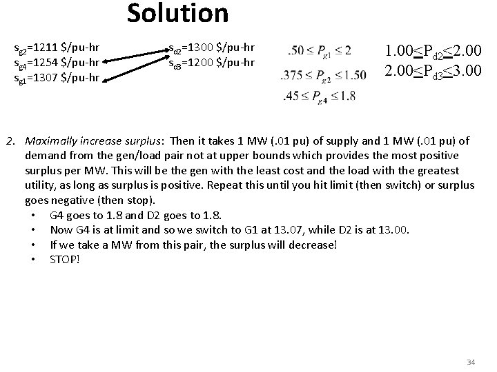
Solution sg 2=1211 $/pu-hr sg 4=1254 $/pu-hr sg 1=1307 $/pu-hr sd 2=1300 $/pu-hr sd 3=1200 $/pu-hr 1. 00<Pd 2<2. 00<Pd 3<3. 00 2. Maximally increase surplus: Then it takes 1 MW (. 01 pu) of supply and 1 MW (. 01 pu) of demand from the gen/load pair not at upper bounds which provides the most positive surplus per MW. This will be the gen with the least cost and the load with the greatest utility, as long as surplus is positive. Repeat this until you hit limit (then switch) or surplus goes negative (then stop). • G 4 goes to 1. 8 and D 2 goes to 1. 8. • Now G 4 is at limit and so we switch to G 1 at 13. 07, while D 2 is at 13. 00. • If we take a MW from this pair, the surplus will decrease! • STOP! 34

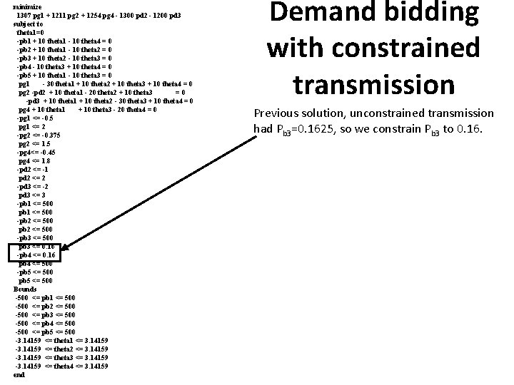
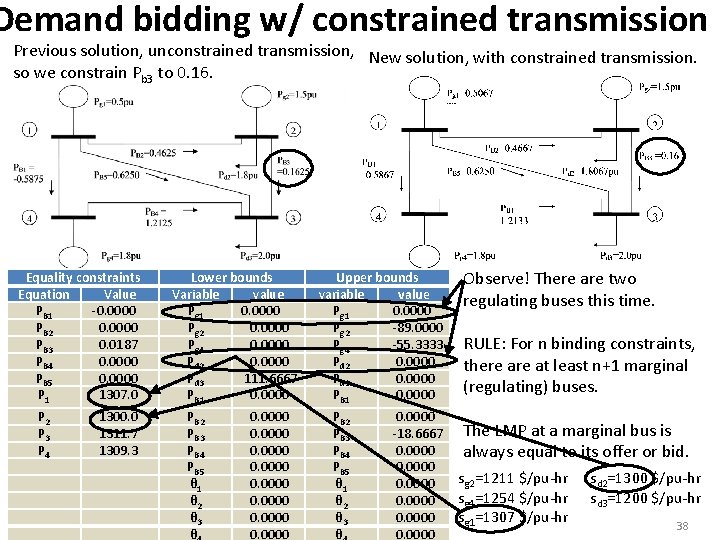
minimize 1307 pg 1 + 1211 pg 2 + 1254 pg 4 - 1300 pd 2 - 1200 pd 3 subject to theta 1=0 -pb 1 + 10 theta 1 - 10 theta 4 = 0 -pb 2 + 10 theta 1 - 10 theta 2 = 0 -pb 3 + 10 theta 2 - 10 theta 3 = 0 -pb 4 - 10 theta 3 + 10 theta 4 = 0 -pb 5 + 10 theta 1 - 10 theta 3 = 0 pg 1 - 30 theta 1 + 10 theta 2 + 10 theta 3 + 10 theta 4 = 0 pg 2 -pd 2 + 10 theta 1 - 20 theta 2 + 10 theta 3 =0 -pd 3 + 10 theta 1 + 10 theta 2 - 30 theta 3 + 10 theta 4 = 0 pg 4 + 10 theta 1 + 10 theta 3 - 20 theta 4 = 0 -pg 1 <= -0. 5 pg 1 <= 2 -pg 2 <= -0. 375 pg 2 <= 1. 5 -pg 4<= -0. 45 pg 4 <= 1. 8 -pd 2 <= -1 pd 2 <= 2 -pd 3 <= -2 pd 3 <= 3 -pb 1 <= 500 -pb 2 <= 500 -pb 3 <= 500 pb 3 <= 0. 16 -pb 4 <= 0. 16 pb 4 <= 500 -pb 5 <= 500 Bounds -500 <= pb 1 <= 500 -500 <= pb 2 <= 500 -500 <= pb 3 <= 500 -500 <= pb 4 <= 500 -500 <= pb 5 <= 500 -3. 14159 <= theta 1 <= 3. 14159 -3. 14159 <= theta 2 <= 3. 14159 -3. 14159 <= theta 3 <= 3. 14159 -3. 14159 <= theta 4 <= 3. 14159 end Demand bidding with constrained transmission Previous solution, unconstrained transmission had Pb 3=0. 1625, so we constrain Pb 3 to 0. 16.

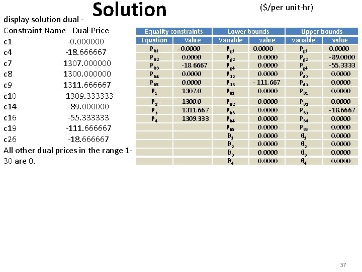
Solution Z*=-$12. 7533 display solution variables Variable Name Solution Value pg 1 0. 506667 pg 2 1. 500000 pg 4 1. 800000 pd 2 1. 806667 pd 3 2. 000000 pb 1 -0. 586667 theta 4 0. 058667 pb 2 0. 466667 theta 2 -0. 046667 pb 3 0. 160000 theta 3 -0. 062667 pb 4 1. 213333 pb 5 0. 626667 All other variables in the range 1 -14 are 0. 36

Solution display solution dual Constraint Name Dual Price c 1 -0. 000000 c 4 -18. 666667 c 7 1307. 000000 c 8 1300. 000000 c 9 1311. 666667 c 10 1309. 333333 c 14 -89. 000000 c 16 -55. 333333 c 19 -111. 666667 c 26 -18. 666667 All other dual prices in the range 130 are 0. ($/per unit-hr) Equality constraints Equation Value PB 1 -0. 0000 PB 2 0. 0000 PB 3 -18. 6667 PB 4 0. 0000 PB 5 0. 0000 P 1 1307. 0 P 2 P 3 P 4 1300. 0 1311. 667 1309. 333 Lower bounds Variable value Pg 1 0. 0000 Pg 2 0. 0000 Pg 4 0. 0000 Pd 2 0. 0000 Pd 3 - 111. 667 PB 1 0. 0000 PB 2 PB 3 PB 4 PB 5 θ 1 θ 2 θ 3 θ 4 0. 0000 0. 0000 Upper bounds variable value Pg 1 0. 0000 Pg 2 -89. 0000 Pg 4 -55. 3333 Pd 2 0. 0000 Pd 3 0. 0000 PB 1 0. 0000 PB 2 PB 3 PB 4 PB 5 θ 1 θ 2 θ 3 θ 4 0. 0000 -18. 6667 0. 0000 37

Demand bidding w/ constrained transmission Previous solution, unconstrained transmission, New solution, with constrained transmission. so we constrain Pb 3 to 0. 16. Equality constraints Equation Value PB 1 -0. 0000 PB 2 0. 0000 PB 3 0. 0187 PB 4 0. 0000 PB 5 0. 0000 P 1 1307. 0 P 2 P 3 P 4 1300. 0 1311. 7 1309. 3 Lower bounds Variable value Pg 1 0. 0000 Pg 2 0. 0000 Pg 4 0. 0000 Pd 2 0. 0000 Pd 3 111. 6667 PB 1 0. 0000 PB 2 PB 3 PB 4 PB 5 θ 1 θ 2 θ 3 θ 0. 0000 0. 0000 Upper bounds variable value Pg 1 0. 0000 Pg 2 -89. 0000 Pg 4 -55. 3333 Pd 2 0. 0000 Pd 3 0. 0000 PB 1 0. 0000 PB 2 PB 3 PB 4 PB 5 θ 1 θ 2 θ 3 θ 0. 0000 -18. 6667 0. 0000 Observe! There are two regulating buses this time. RULE: For n binding constraints, there at least n+1 marginal (regulating) buses. The LMP at a marginal bus is always equal to its offer or bid. sg 2=1211 $/pu-hr sd 2=1300 $/pu-hr sg 4=1254 $/pu-hr sd 3=1200 $/pu-hr sg 1=1307 $/pu-hr 38

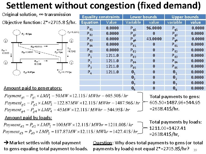
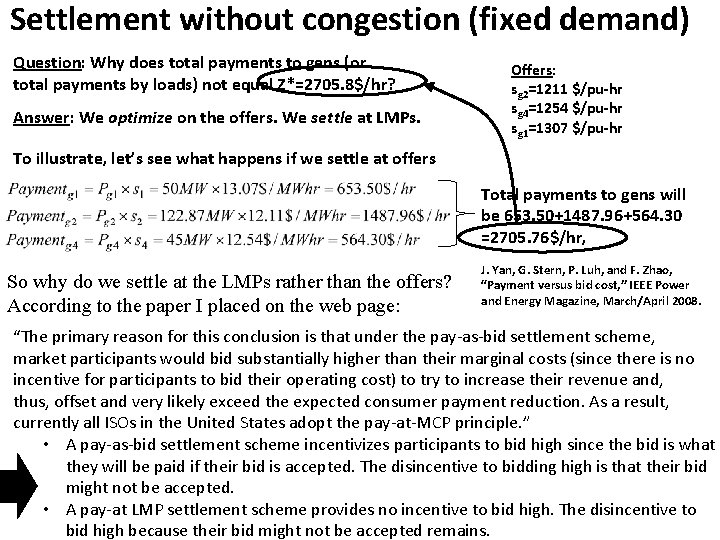
Settlement without congestion (fixed demand) Original solution, ∞ transmission Equality constraints Value Objective function: Z*=2705. 8 $/hr. Equation PB 1 0. 0000 PB 2 0. 0000 PB 3 0. 0000 PB 4 0. 0000 PB 5 0. 0000 P 1 1211. 0 P 2 1211. 0 P 3 1211. 0 P 4 1211. 0 Amount paid to generators: Lower bounds Variable value Pg 1 96. 0000 Pg 2 0 Pg 4 43. 0000 PB 1 0 PB 2 0 PB 3 0 PB 4 0 PB 5 0 θ 1 0 θ 2 0 θ 3 0 θ 4 0 Upper bounds variable value Pg 1 0. 0000 Pg 2 0. 0000 Pg 4 0. 0000 PB 1 0. 0000 PB 2 0. 0000 PB 3 0. 0000 PB 4 0. 0000 PB 5 0. 0000 θ 1 0. 0000 θ 2 0. 0000 θ 3 0. 0000 θ 4 0. 0000 Total payments to gens: 605. 50+1487. 96+544. 95 =2638. 41$/hr. Amount paid by loads: Total payments by loads: 1211. 00+1427. 41 =2638. 41$/hr, Market settles with total payment Question: Why does total payments to gens (or total to gens equaling total payment to loads. payments by loads) not equal Z*=2705. 8$/hr? 39

Settlement without congestion (fixed demand) Question: Why does total payments to gens (or total payments by loads) not equal Z*=2705. 8$/hr? Answer: We optimize on the offers. We settle at LMPs. Offers: sg 2=1211 $/pu-hr sg 4=1254 $/pu-hr sg 1=1307 $/pu-hr To illustrate, let’s see what happens if we settle at offers Total payments to gens will be 653. 50+1487. 96+564. 30 =2705. 76$/hr, So why do we settle at the LMPs rather than the offers? According to the paper I placed on the web page: J. Yan, G. Stern, P. Luh, and F. Zhao, “Payment versus bid cost, ” IEEE Power and Energy Magazine, March/April 2008. “The primary reason for this conclusion is that under the pay-as-bid settlement scheme, market participants would bid substantially higher than their marginal costs (since there is no incentive for participants to bid their operating cost) to try to increase their revenue and, thus, offset and very likely exceed the expected consumer payment reduction. As a result, currently all ISOs in the United States adopt the pay-at-MCP principle. ” • A pay-as-bid settlement scheme incentivizes participants to bid high since the bid is what they will be paid if their bid is accepted. The disincentive to bidding high is that their bid might not be accepted. • A pay-at LMP settlement scheme provides no incentive to bid high. The disincentive to bid high because their bid might not be accepted remains.

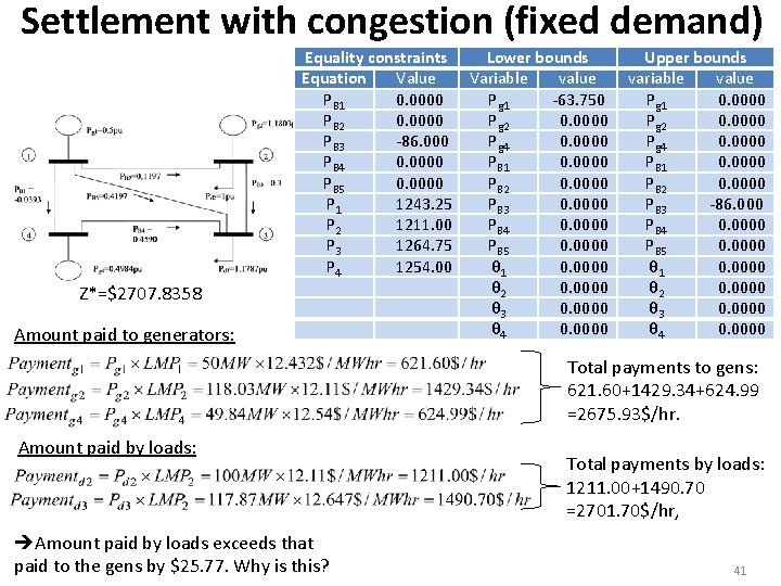
Settlement with congestion (fixed demand) Z*=$2707. 8358 Amount paid to generators: Equality constraints Lower bounds Equation Value Variable value PB 1 0. 0000 Pg 1 -63. 750 PB 2 0. 0000 Pg 2 0. 0000 PB 3 -86. 000 Pg 4 0. 0000 PB 1 0. 0000 PB 5 0. 0000 PB 2 0. 0000 P 1 1243. 25 PB 3 0. 0000 P 2 1211. 00 PB 4 0. 0000 P 3 1264. 75 PB 5 0. 0000 P 4 1254. 00 θ 1 0. 0000 θ 2 0. 0000 θ 3 0. 0000 θ 4 0. 0000 Upper bounds variable value Pg 1 0. 0000 Pg 2 0. 0000 Pg 4 0. 0000 PB 1 0. 0000 PB 2 0. 0000 PB 3 -86. 000 PB 4 0. 0000 PB 5 0. 0000 θ 1 0. 0000 θ 2 0. 0000 θ 3 0. 0000 θ 4 0. 0000 Total payments to gens: 621. 60+1429. 34+624. 99 =2675. 93$/hr. Amount paid by loads: Amount paid by loads exceeds that paid to the gens by $25. 77. Why is this? Total payments by loads: 1211. 00+1490. 70 =2701. 70$/hr, 41

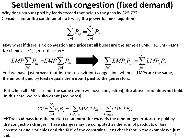
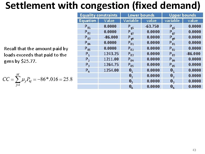
Settlement with congestion (fixed demand) Why does amount paid by loads exceed that paid to the gens by $25. 77? Consider under the condition of no losses, the power balance equation: Now what if there is no congestion and prices at all buses are the same at LMP, i. e. , LMP j=LMP for all buses j=1, …, n. In this case: And we have just proved that for the case without congestion, when all LMPs are the same, the amount paid by loads equals the amount paid to the generators. But when all LMPs are not the same (when we have congestion), the above proof does not hold. In this case, we can show that (see notes): The load pays into the market an amount the exceeds the amount generators are paid by the congestion charges. These charges may be computed as the sum of products of line constraint dual variables and the RHS of the constraint. Let’s check that in the example we just 42 did.

Settlement with congestion (fixed demand) Recall that the amount paid by loads exceeds that paid to the gens by $25. 77. Equality constraints Lower bounds Equation Value Variable value PB 1 0. 0000 Pg 1 -63. 750 PB 2 0. 0000 Pg 2 0. 0000 PB 3 -86. 000 Pg 4 0. 0000 PB 1 0. 0000 PB 5 0. 0000 PB 2 0. 0000 P 1 1243. 25 PB 3 0. 0000 P 2 1211. 00 PB 4 0. 0000 P 3 1264. 75 PB 5 0. 0000 P 4 1254. 00 θ 1 0. 0000 θ 2 0. 0000 θ 3 0. 0000 θ 4 0. 0000 Upper bounds variable value Pg 1 0. 0000 Pg 2 0. 0000 Pg 4 0. 0000 PB 1 0. 0000 PB 2 0. 0000 PB 3 -86. 000 PB 4 0. 0000 PB 5 0. 0000 θ 1 0. 0000 θ 2 0. 0000 θ 3 0. 0000 θ 4 0. 0000 43

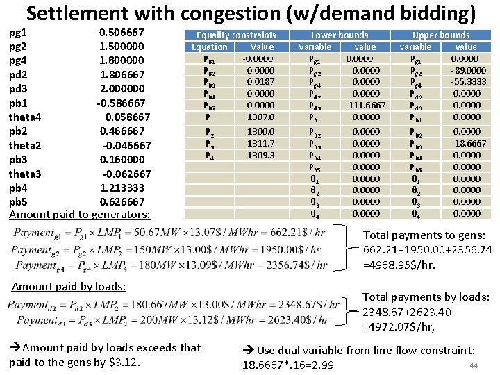
Settlement with congestion (w/demand bidding) pg 1 pg 2 pg 4 pd 2 pd 3 pb 1 theta 4 pb 2 theta 2 pb 3 theta 3 pb 4 pb 5 0. 506667 1. 500000 1. 806667 2. 000000 -0. 586667 0. 058667 0. 466667 -0. 046667 0. 160000 -0. 062667 1. 213333 0. 626667 Amount paid to generators: Equality constraints Equation Value PB 1 -0. 0000 PB 2 0. 0000 PB 3 0. 0187 PB 4 0. 0000 PB 5 0. 0000 P 1 1307. 0 P 2 P 3 P 4 1300. 0 1311. 7 1309. 3 Lower bounds Variable value Pg 1 0. 0000 Pg 2 0. 0000 Pg 4 0. 0000 Pd 2 0. 0000 Pd 3 111. 6667 PB 1 0. 0000 PB 2 PB 3 PB 4 PB 5 θ 1 θ 2 θ 3 θ 4 0. 0000 0. 0000 Upper bounds variable value Pg 1 0. 0000 Pg 2 -89. 0000 Pg 4 -55. 3333 Pd 2 0. 0000 Pd 3 0. 0000 PB 1 0. 0000 PB 2 PB 3 PB 4 PB 5 θ 1 θ 2 θ 3 θ 4 0. 0000 -18. 6667 0. 0000 Total payments to gens: 662. 21+1950. 00+2356. 74 =4968. 95$/hr. Amount paid by loads: Amount paid by loads exceeds that paid to the gens by $3. 12. Total payments by loads: 2348. 67+2623. 40 =4972. 07$/hr, Use dual variable from line flow constraint: 44 18. 6667*. 16=2. 99

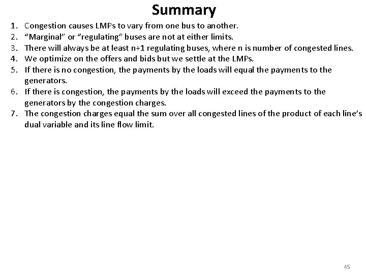
Summary 1. 2. 3. 4. 5. Congestion causes LMPs to vary from one bus to another. “Marginal” or “regulating” buses are not at either limits. There will always be at least n+1 regulating buses, where n is number of congested lines. We optimize on the offers and bids but we settle at the LMPs. If there is no congestion, the payments by the loads will equal the payments to the generators. 6. If there is congestion, the payments by the loads will exceed the payments to the generators by the congestion charges. 7. The congestion charges equal the sum over all congested lines of the product of each line’s dual variable and its line flow limit. 45