EEEcon 458 The Simplex Method J Mc Calley

EE/Econ 458 The Simplex Method J. Mc. Calley 1

An approach 2

Definitions Adjacent corner points are connected by a single line segment on the boundary of the feasible region. One corner point is better than another if it has a higher value of the objective function f. 3

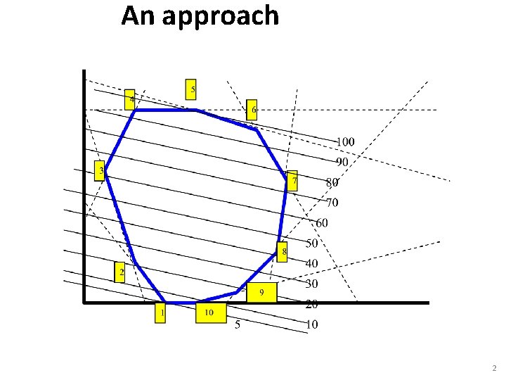
An approach 1. Pick a corner point at random. 2. Move to an adjacent corner point that is better. a. If there are two that are better, move to the one that is best. b. If there are no better adjacent corner points, the current corner point is the solution to the problem. Optimality (stopping) condition: If a corner point feasible solution is equal to or better than all its adjacent corner point feasible solutions, then it is equal to or better than all other corner point feasible solutions, i. e. , it is optimal. Main ideas of proof: 1. If objective function monotonically increases (decreases) in some direction within the decision-vector space, then each adjacent corner point will become progressively better in the direction of objective function increase (decrease) such that the last corner point must have two adjacent corner points that are worse. 2. The monotonicity of objective function increase (decrease) is guaranteed by its linearity. 4

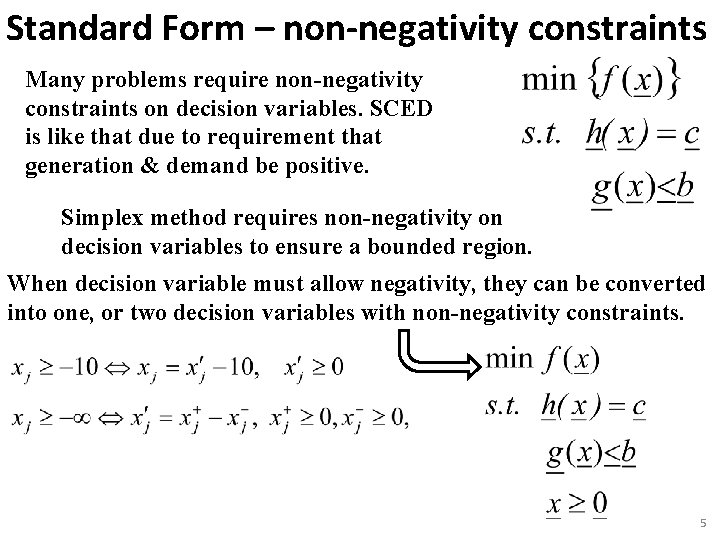
Standard Form – non-negativity constraints Many problems require non-negativity constraints on decision variables. SCED is like that due to requirement that generation & demand be positive. Simplex method requires non-negativity on decision variables to ensure a bounded region. When decision variable must allow negativity, they can be converted into one, or two decision variables with non-negativity constraints. 5

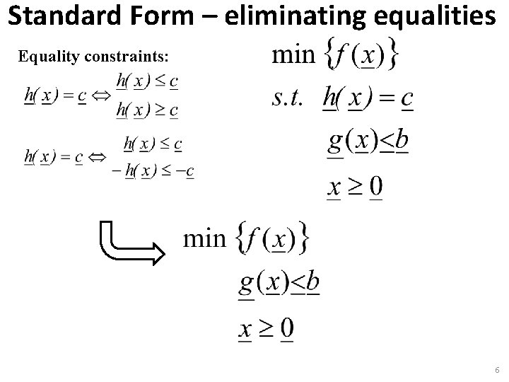
Standard Form – eliminating equalities Equality constraints: 6

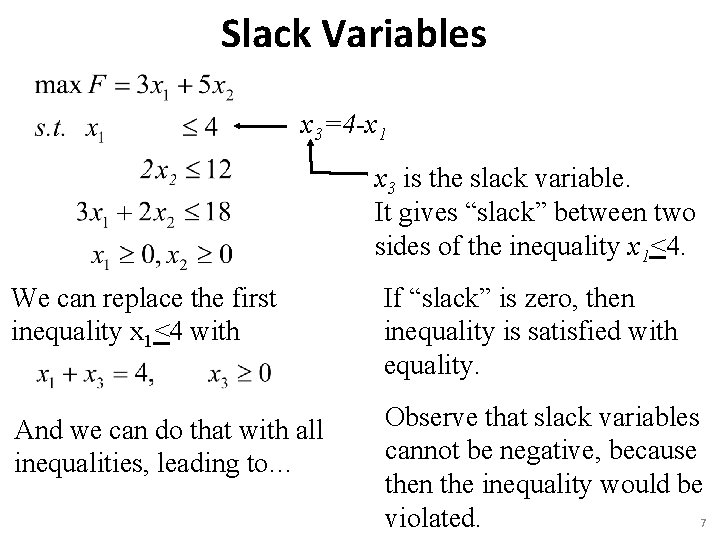
Slack Variables x 3=4 -x 1 x 3 is the slack variable. It gives “slack” between two sides of the inequality x 1<4. We can replace the first inequality x 1<4 with If “slack” is zero, then inequality is satisfied with equality. And we can do that with all inequalities, leading to… Observe that slack variables cannot be negative, because then the inequality would be violated. 7

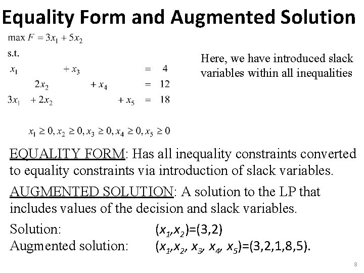
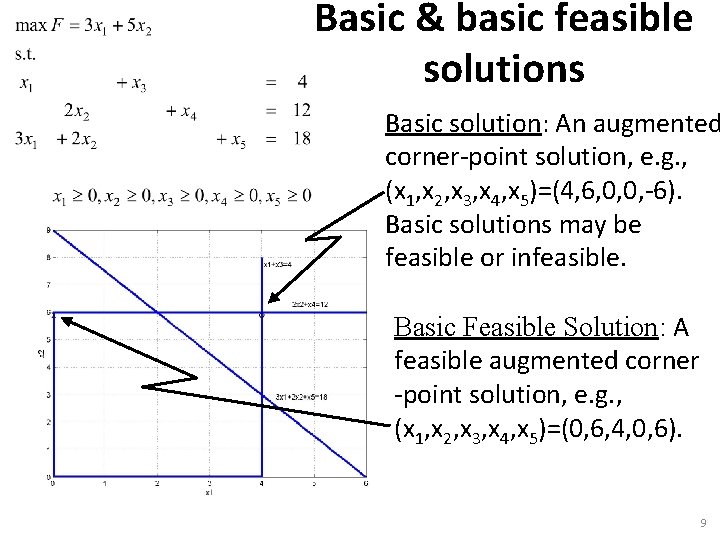
Equality Form and Augmented Solution Here, we have introduced slack variables within all inequalities EQUALITY FORM: Has all inequality constraints converted to equality constraints via introduction of slack variables. AUGMENTED SOLUTION: A solution to the LP that includes values of the decision and slack variables. Solution: (x 1, x 2)=(3, 2) Augmented solution: (x 1, x 2, x 3, x 4, x 5)=(3, 2, 1, 8, 5). 8

Basic & basic feasible solutions Basic solution: An augmented corner-point solution, e. g. , (x 1, x 2, x 3, x 4, x 5)=(4, 6, 0, 0, -6). Basic solutions may be feasible or infeasible. Basic Feasible Solution: A feasible augmented corner -point solution, e. g. , (x 1, x 2, x 3, x 4, x 5)=(0, 6, 4, 0, 6). 9

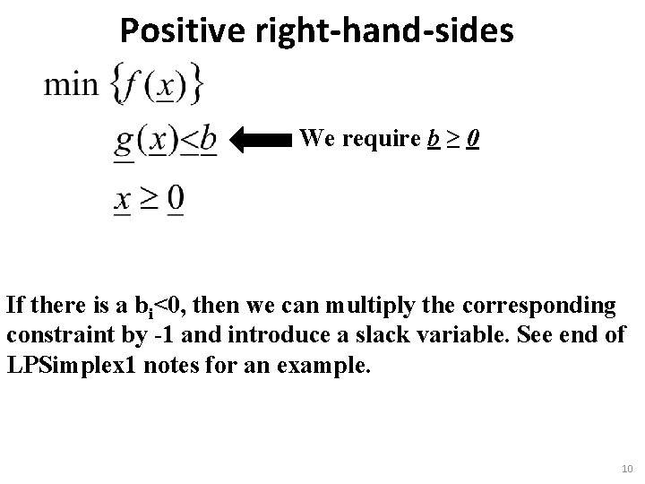
Positive right-hand-sides We require b ≥ 0 If there is a bi<0, then we can multiply the corresponding constraint by -1 and introduce a slack variable. See end of LPSimplex 1 notes for an example. 10

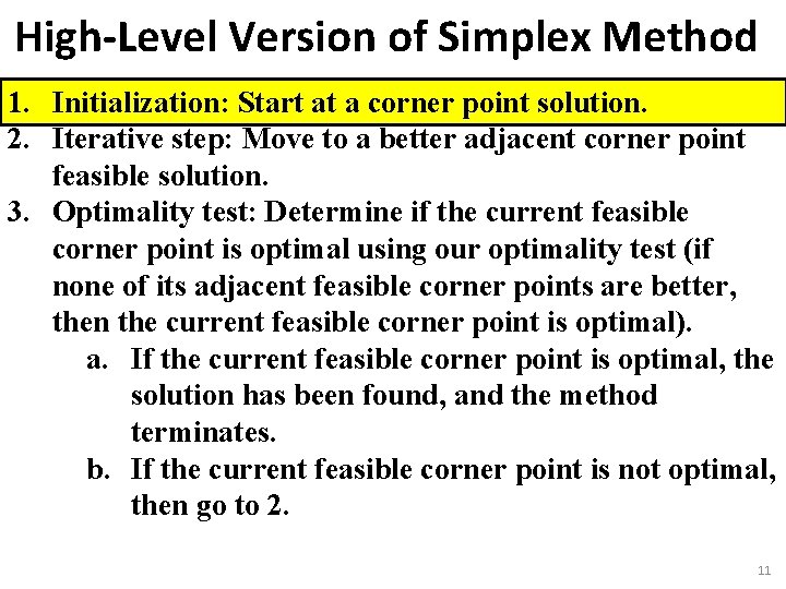
High-Level Version of Simplex Method 1. Initialization: Start at a corner point solution. 2. Iterative step: Move to a better adjacent corner point feasible solution. 3. Optimality test: Determine if the current feasible corner point is optimal using our optimality test (if none of its adjacent feasible corner points are better, then the current feasible corner point is optimal). a. If the current feasible corner point is optimal, the solution has been found, and the method terminates. b. If the current feasible corner point is not optimal, then go to 2. 11

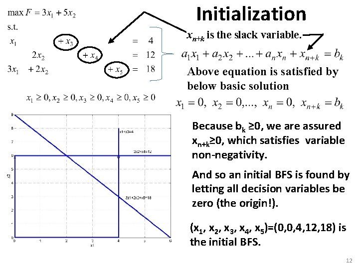
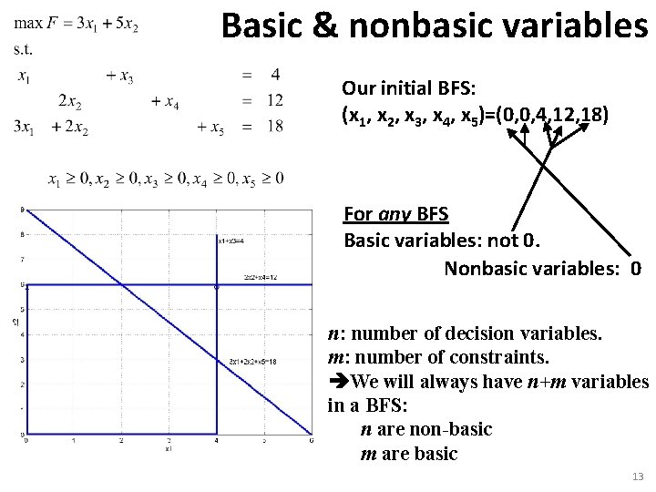
Initialization xn+k is the slack variable. Above equation is satisfied by below basic solution Because bk ≥ 0, we are assured xn+k≥ 0, which satisfies variable non-negativity. And so an initial BFS is found by letting all decision variables be zero (the origin!). (x 1, x 2, x 3, x 4, x 5)=(0, 0, 4, 12, 18) is the initial BFS. 12

Basic & nonbasic variables Our initial BFS: (x 1, x 2, x 3, x 4, x 5)=(0, 0, 4, 12, 18) For any BFS Basic variables: not 0. Nonbasic variables: 0 n: number of decision variables. m: number of constraints. We will always have n+m variables in a BFS: n are non-basic m are basic 13

High-Level Version of Simplex Method 1. Initialization: Start at a corner point solution. 2. Iterative step: Move to a better adjacent corner point feasible solution. 3. Optimality test: Determine if the current feasible corner point is optimal using our optimality test (if none of its adjacent feasible corner points are better, then the current feasible corner point is optimal). a. If the current feasible corner point is optimal, the solution has been found, and the method terminates. b. If the current feasible corner point is not optimal, then go to 2. 14

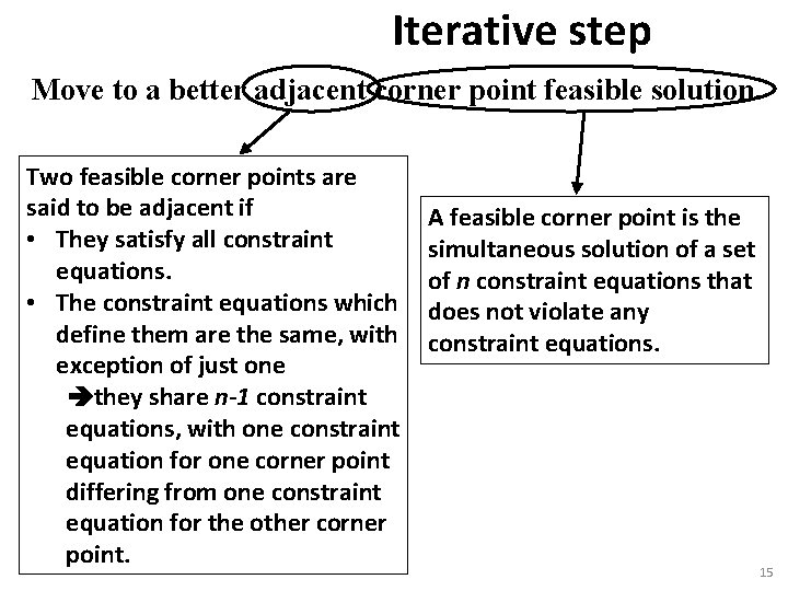
Iterative step Move to a better adjacent corner point feasible solution. Two feasible corner points are said to be adjacent if • They satisfy all constraint equations. • The constraint equations which define them are the same, with exception of just one they share n-1 constraint equations, with one constraint equation for one corner point differing from one constraint equation for the other corner point. A feasible corner point is the simultaneous solution of a set of n constraint equations that does not violate any constraint equations. 15

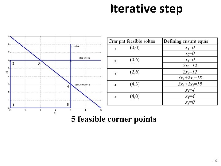
Iterative step 5 feasible corner points 16

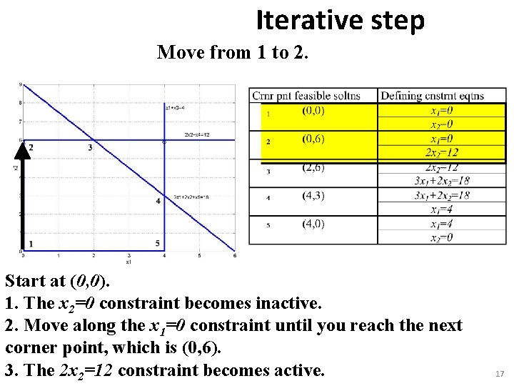
Iterative step Move from 1 to 2. Start at (0, 0). 1. The x 2=0 constraint becomes inactive. 2. Move along the x 1=0 constraint until you reach the next corner point, which is (0, 6). 3. The 2 x 2=12 constraint becomes active. 17

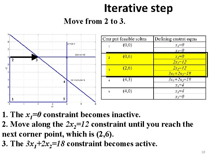
Iterative step Move from 2 to 3. 1. The x 1=0 constraint becomes inactive. 2. Move along the 2 x 2=12 constraint until you reach the next corner point, which is (2, 6). 3. The 3 x 1+2 x 2=18 constraint becomes active. 18

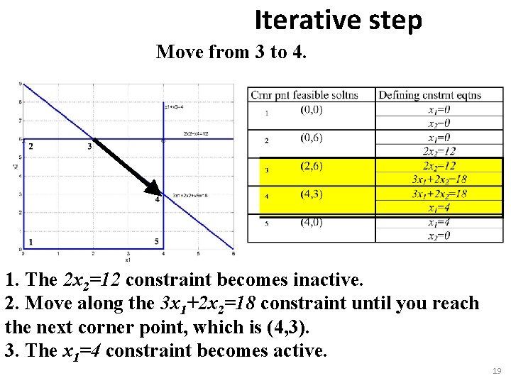
Iterative step Move from 3 to 4. 1. The 2 x 2=12 constraint becomes inactive. 2. Move along the 3 x 1+2 x 2=18 constraint until you reach the next corner point, which is (4, 3). 3. The x 1=4 constraint becomes active. 19

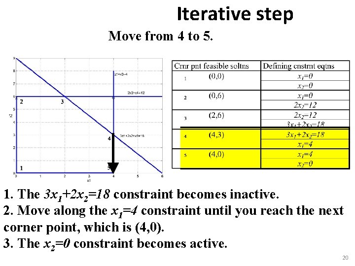
Iterative step Move from 4 to 5. 1. The 3 x 1+2 x 2=18 constraint becomes inactive. 2. Move along the x 1=4 constraint until you reach the next corner point, which is (4, 0). 3. The x 2=0 constraint becomes active. 20

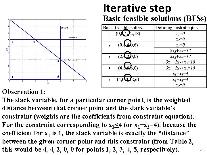
Iterative step Basic feasible solutions (BFSs) Observation 1: The slack variable, for a particular corner point, is the weighted distance between that corner point and the slack variable’s constraint (weights are the coefficients from constraint equation). For the constraint corresponding to x 1<4 (or x 1+x 3=4), because the coefficient for x 1 is 1, the slack variable is exactly the “distance” between the given corner point and this constraint (from Table 2, this would be 4, 4, 2, 0, 0 for points 1, 2, 3, 4, 5, respectively). 21

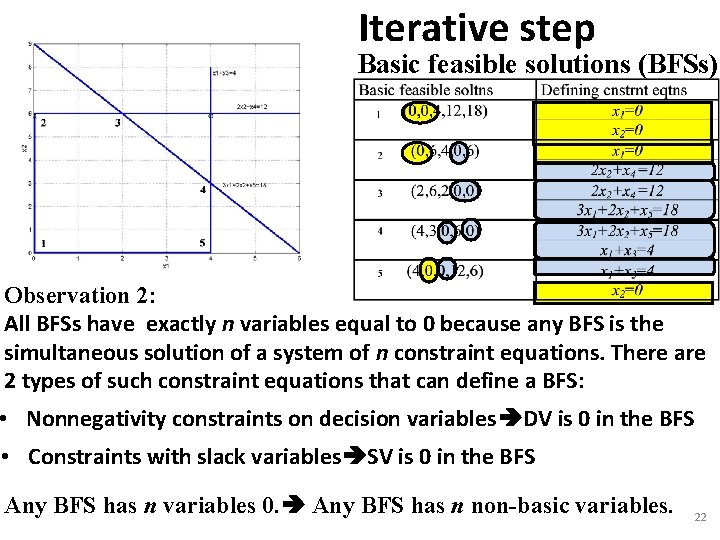
Iterative step Basic feasible solutions (BFSs) Observation 2: All BFSs have exactly n variables equal to 0 because any BFS is the simultaneous solution of a system of n constraint equations. There are 2 types of such constraint equations that can define a BFS: • Nonnegativity constraints on decision variables DV is 0 in the BFS • Constraints with slack variables SV is 0 in the BFS Any BFS has n variables 0. Any BFS has n non-basic variables. 22

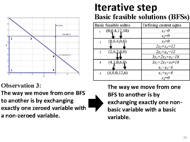
Iterative step Basic feasible solutions (BFSs) Observation 3: The way we move from one BFS to another is by exchanging exactly one zeroed variable with a non-zeroed variable. The way we move from one BFS to another is by exchanging exactly one nonbasic variable with a basic variable. 23

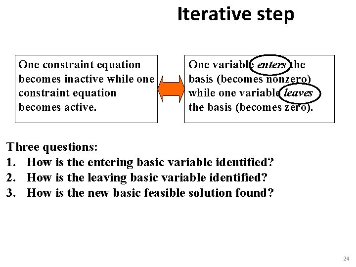
Iterative step One constraint equation becomes inactive while one constraint equation becomes active. One variable enters the basis (becomes nonzero) while one variable leaves the basis (becomes zero). Three questions: 1. How is the entering basic variable identified? 2. How is the leaving basic variable identified? 3. How is the new basic feasible solution found? 24

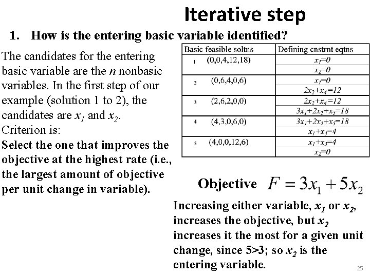
Iterative step 1. How is the entering basic variable identified? The candidates for the entering basic variable are the n nonbasic variables. In the first step of our example (solution 1 to 2), the candidates are x 1 and x 2. Criterion is: Select the one that improves the objective at the highest rate (i. e. , the largest amount of objective per unit change in variable). Objective Increasing either variable, x 1 or x 2, increases the objective, but x 2 increases it the most for a given unit change, since 5>3; so x 2 is the entering variable. 25

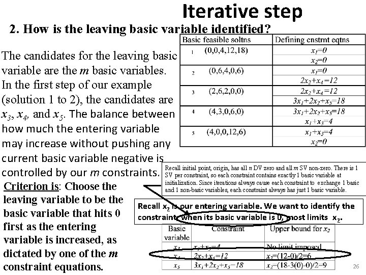
Iterative step 2. How is the leaving basic variable identified? The candidates for the leaving basic variable are the m basic variables. In the first step of our example (solution 1 to 2), the candidates are x 3, x 4, and x 5. The balance between how much the entering variable may increase without pushing any current basic variable negative is Recall initial point, origin, has all n DV zero and all m SV non-zero. There is 1 controlled by our m constraints. SV per constraint, so each constraint contains exactly 1 basic variable at Criterion is: Choose the leaving variable to be the basic variable that hits 0 first as the entering variable is increased, as dictated by one of the m constraint equations. initialization. Since iterations always cause each constraint to exchange 1 basic and 1 non-basic variables, each constraint always has just 1 basic variable. Recall x 2 is our entering variable. We want to identify the constraint, when its basic variable is 0, most limits x 2. 26

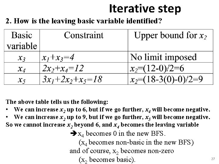
Iterative step 2. How is the leaving basic variable identified? The above table tells us the following: • We can increase x 2 up to 6, but if we go further, x 4 will become negative. • We can increase x 2 up to 9, but if we go further, x 5 will become negative. So we cannot increase x 2 beyond 6, and x 4 becomes the leaving variable è x 4 becomes 0 in the new BFS. (x 4 becomes non-basic in the new BFS) and of course, x 2 becomes non-zero (x 2 becomes basic). 27

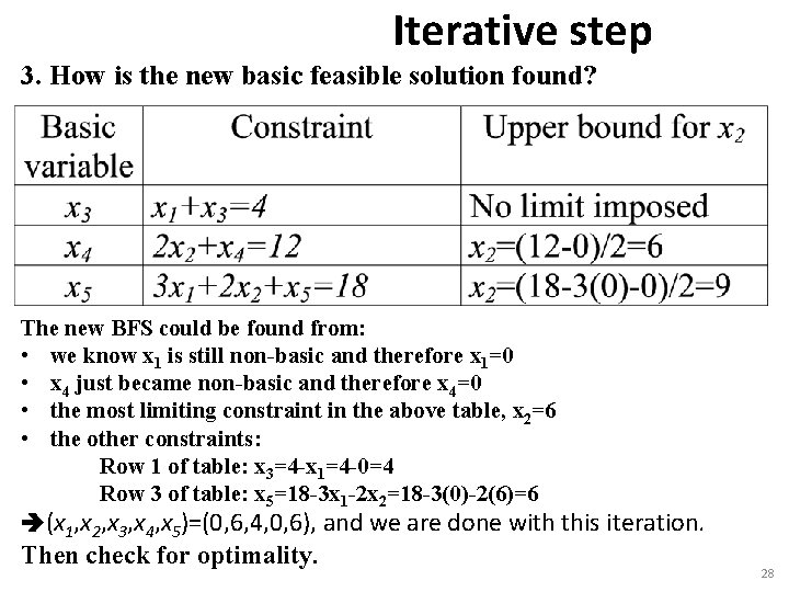
Iterative step 3. How is the new basic feasible solution found? The new BFS could be found from: • we know x 1 is still non-basic and therefore x 1=0 • x 4 just became non-basic and therefore x 4=0 • the most limiting constraint in the above table, x 2=6 • the other constraints: Row 1 of table: x 3=4 -x 1=4 -0=4 Row 3 of table: x 5=18 -3 x 1 -2 x 2=18 -3(0)-2(6)=6 (x 1, x 2, x 3, x 4, x 5)=(0, 6, 4, 0, 6), and we are done with this iteration. Then check for optimality. 28

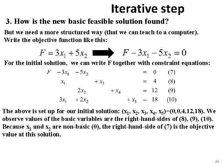
Iterative step 3. How is the new basic feasible solution found? But we need a more structured way (that we can teach to a computer). Write the objective function like this: For the initial solution, we can write F together with constraint equations: The above is set up for our initial solution: (x 1, x 2, x 3, x 4, x 5)=(0, 0, 4, 12, 18). We observe values of the basic variables are the right-hand-sides of (8), (9), (10). Because x 1 and x 2 are non-basic (0), the right-hand-side of (7) is the objective value at this solution. 29

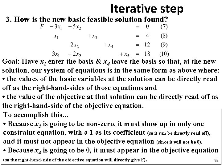
Iterative step 3. How is the new basic feasible solution found? Goal: Have x 2 enter the basis & x 4 leave the basis so that, at the new solution, our system of equations is in the same form as above where: • the values of the basic variables at the solution can be directly read off as the right-hand-sides of those equations and • the value of the objective at that solution can be directly read off as the right-hand-side of the objective equation. To accomplish this… • Because x 2 is going to be non-zero, it must show up in only one constraint equation, with a 1 as its coefficient (so it can be directly read off), and it must not appear in the objective equation (since it will not be 0). • Because x 4 is going to be 0, it must appear in the objective equation (so the right-hand-side of the objective equation will directly give F). 30

Iterative step 3. How is the new basic feasible solution found? Entering variable: x 2 Leaving variable: x 4 We want to eliminate (make 0) the coefficient of x 2 (-5) in row 1. We will use row 3 as our “pivot row” (and a 33 our pivot) so that the leaving variable (x 4) appears in row 1 after eliminating x 2. 31

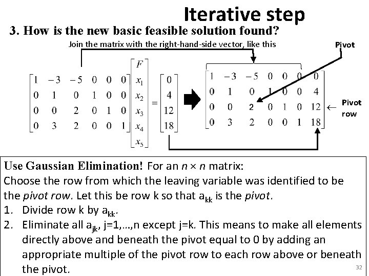
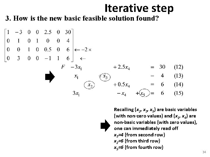
Iterative step 3. How is the new basic feasible solution found? Join the matrix with the right-hand-side vector, like this Pivot row Use Gaussian Elimination! For an n × n matrix: Choose the row from which the leaving variable was identified to be the pivot row. Let this be row k so that akk is the pivot. 1. Divide row k by akk. 2. Eliminate all ajk, j=1, …, n except j=k. This means to make all elements directly above and beneath the pivot equal to 0 by adding an appropriate multiple of the pivot row to each row above or beneath 32 the pivot.

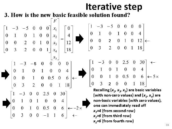
Iterative step 3. How is the new basic feasible solution found? Recalling (x 2, x 3, x 5) are basic variables (with non-zero values) and (x 1, x 4) are non-basic variables (with zero values), one can immediately read off x 3=4 (from second row) x 2=6 (from third row) x 5=6 (from fourth row) 33

Iterative step 3. How is the new basic feasible solution found? Recalling (x 2, x 3, x 5) are basic variables (with non-zero values) and (x 1, x 4) are non-basic variables (with zero values), one can immediately read off x 3=4 (from second row) x 2=6 (from third row) x 5=6 (from fourth row) 34

Iterative step – Key ideas How to identify the entering variable? Select the variable that improves the objective at the highest rate (i. e. , the largest amount of objective per unit change in variable). How to identify the leaving variable? Choose the leaving variable to be the one that hits 0 first as the entering variable is increased, as dictated by one of the m constraint equations. How is the new BFS found? Using the equation used to identify the leaving variable as the pivot row, eliminate the entering variable from all other equations. 35

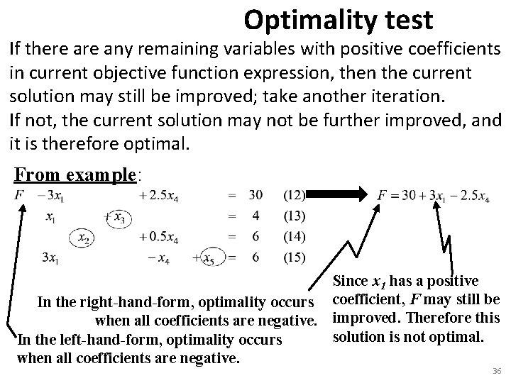
Optimality test If there any remaining variables with positive coefficients in current objective function expression, then the current solution may still be improved; take another iteration. If not, the current solution may not be further improved, and it is therefore optimal. From example: Since x 1 has a positive In the right-hand-form, optimality occurs coefficient, F may still be when all coefficients are negative. improved. Therefore this solution is not optimal. In the left-hand-form, optimality occurs when all coefficients are negative. 36