EEEcon 458 Duality J Mc Calley 1 HW5

EE/Econ 458 Duality J. Mc. Calley 1

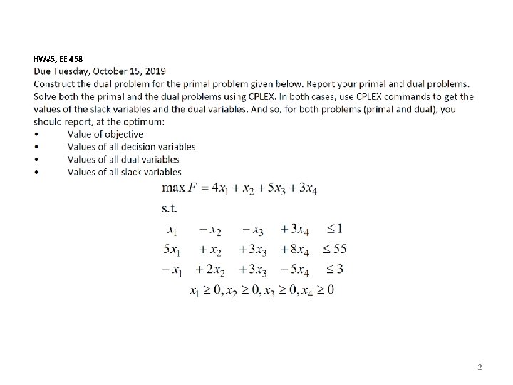
HW#5, EE 458 2

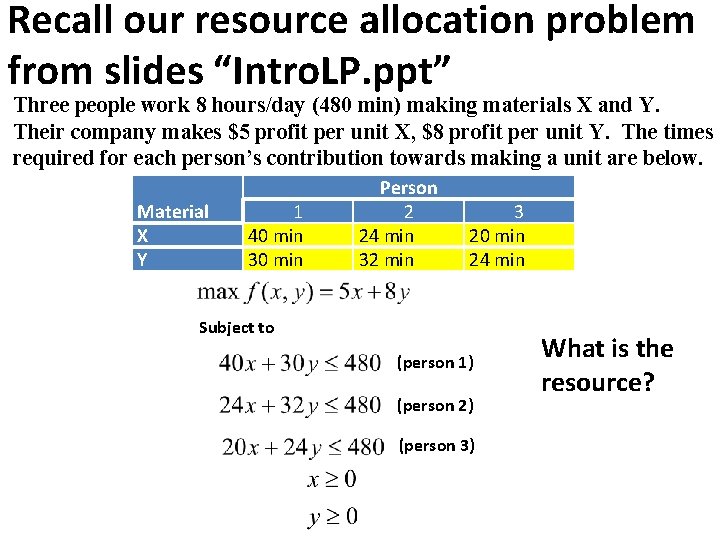
Recall our resource allocation problem from slides “Intro. LP. ppt” Three people work 8 hours/day (480 min) making materials X and Y. Their company makes $5 profit per unit X, $8 profit per unit Y. The times required for each person’s contribution towards making a unit are below. Material X Y 1 40 min 30 min Person 2 24 min 32 min 3 20 min 24 min Subject to (person 1) (person 2) (person 3) What is the resource?

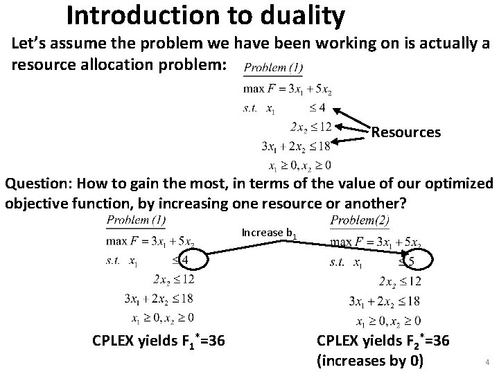
Introduction to duality Let’s assume the problem we have been working on is actually a resource allocation problem: Resources Question: How to gain the most, in terms of the value of our optimized objective function, by increasing one resource or another? Increase b 1 CPLEX yields F 1*=36 CPLEX yields F 2*=36 (increases by 0) 4

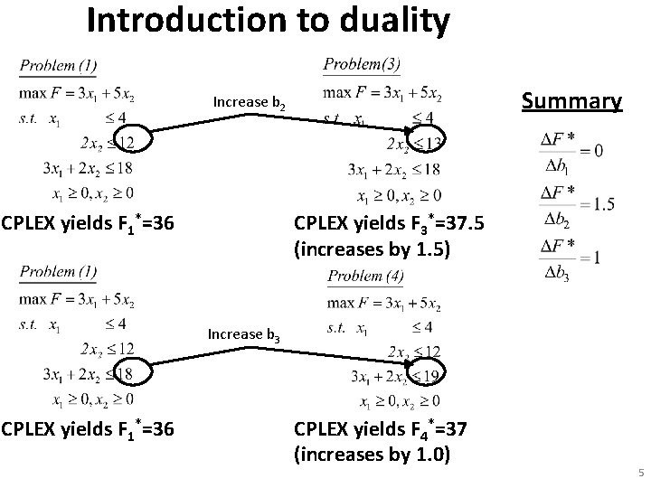
Introduction to duality Summary Increase b 2 CPLEX yields F 1*=36 CPLEX yields F 3*=37. 5 (increases by 1. 5) Increase b 3 CPLEX yields F 1*=36 CPLEX yields F 4*=37 (increases by 1. 0) 5

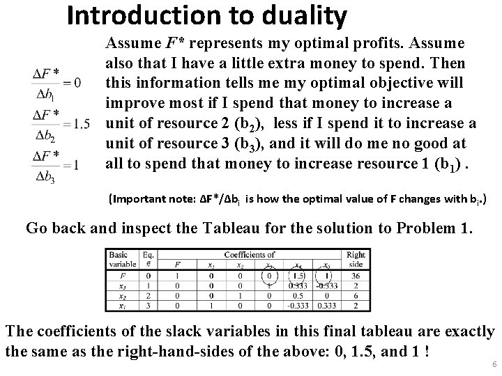
Introduction to duality Assume F* represents my optimal profits. Assume also that I have a little extra money to spend. Then this information tells me my optimal objective will improve most if I spend that money to increase a unit of resource 2 (b 2), less if I spend it to increase a unit of resource 3 (b 3), and it will do me no good at all to spend that money to increase resource 1 (b 1). (Important note: ΔF*/Δbi is how the optimal value of F changes with bi. ) Go back and inspect the Tableau for the solution to Problem 1. The coefficients of the slack variables in this final tableau are exactly the same as the right-hand-sides of the above: 0, 1. 5, and 1 ! 6

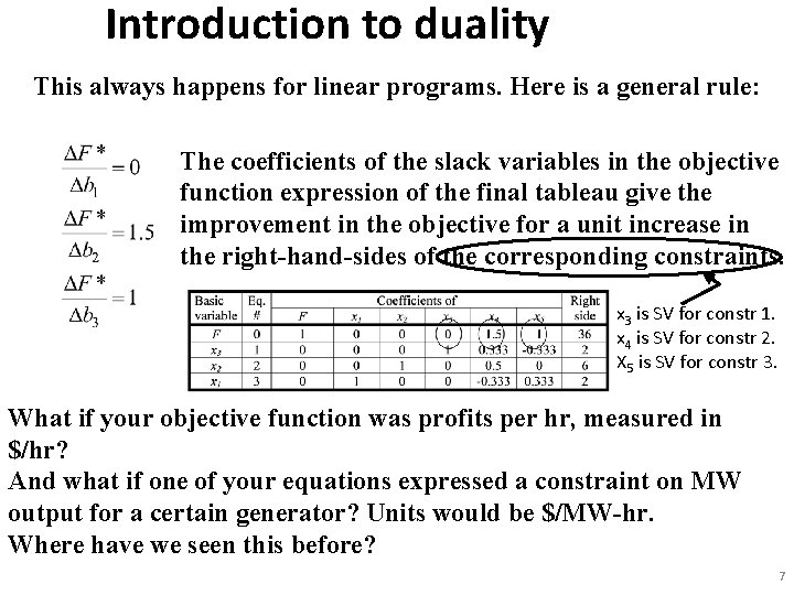
Introduction to duality This always happens for linear programs. Here is a general rule: The coefficients of the slack variables in the objective function expression of the final tableau give the improvement in the objective for a unit increase in the right-hand-sides of the corresponding constraints. x 3 is SV for constr 1. x 4 is SV for constr 2. X 5 is SV for constr 3. What if your objective function was profits per hr, measured in $/hr? And what if one of your equations expressed a constraint on MW output for a certain generator? Units would be $/MW-hr. Where have we seen this before? 7

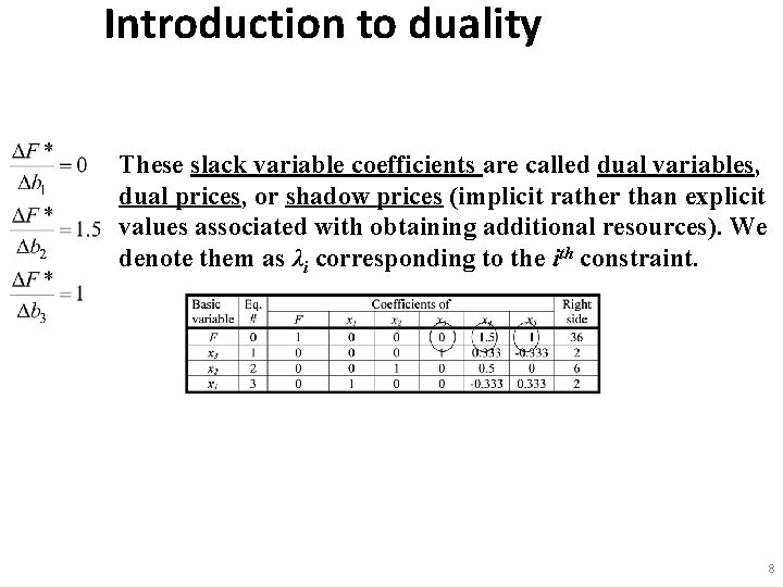
Introduction to duality These slack variable coefficients are called dual variables, dual prices, or shadow prices (implicit rather than explicit values associated with obtaining additional resources). We denote them as λi corresponding to the ith constraint. 8

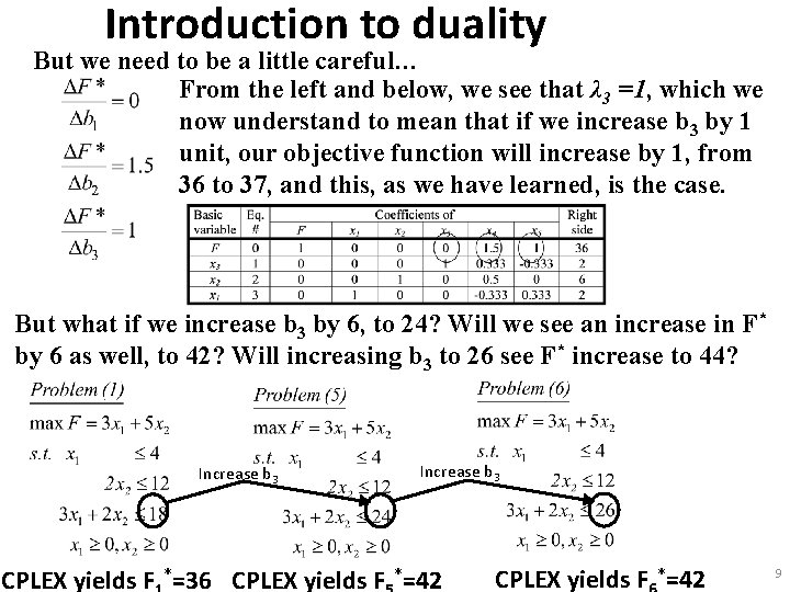
Introduction to duality But we need to be a little careful… From the left and below, we see that λ 3 =1, which we now understand to mean that if we increase b 3 by 1 unit, our objective function will increase by 1, from 36 to 37, and this, as we have learned, is the case. But what if we increase b 3 by 6, to 24? Will we see an increase in F* by 6 as well, to 42? Will increasing b 3 to 26 see F* increase to 44? Increase b 3 CPLEX yields F *=36 CPLEX yields F *=42 9

Introduction to duality There are two observations to be made here: 1. Changing some bi does not influence F*. Only a subset of resources limit the objective. You may have labor hours, trucks, & pipe fittings as resources, each of which are individually constrained. You have a large truck fleet and a whole warehouse of pipe fittings, but you don’t have enough labor. And so you increase labor until you hit the limit on pipe fitting inventory. You then increase pipe fitting inventory, but soon you hit the limit on trucks. 2. ΔF*/Δbi is not accurate if Δbi gets too large. A better definition of the dual variables follows… (next slide) 10

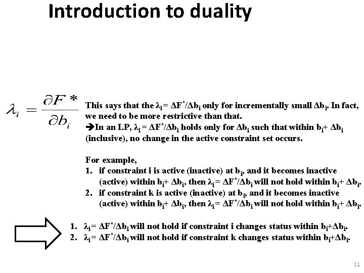
Introduction to duality This says that the λi = ΔF*/Δbi only for incrementally small Δbi. In fact, we need to be more restrictive than that. In an LP, λi = ΔF*/Δbi holds only for Δbi such that within bi+ Δbi (inclusive), no change in the active constraint set occurs. For example, 1. if constraint i is active (inactive) at bi, and it becomes inactive (active) within bi+ Δbi, then λi = ΔF*/Δbi will not hold within bi+ Δbi. 2. if constraint k is active (inactive) at bi, and it becomes inactive (active) within bi+ Δbi, then λi = ΔF*/Δbi will not hold within bi+ Δbi. 1. λi = ΔF*/Δbi will not hold if constraint i changes status within bi+Δbi. 2. λi = ΔF*/Δbi will not hold if constraint k changes status within bi+Δbi. 11

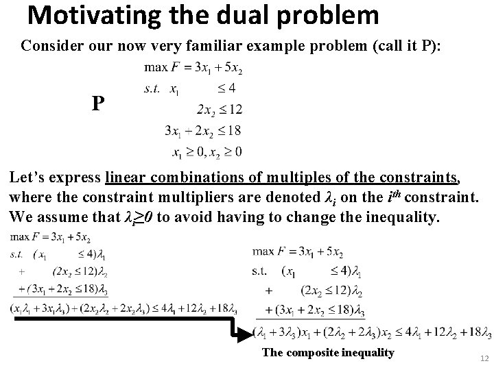
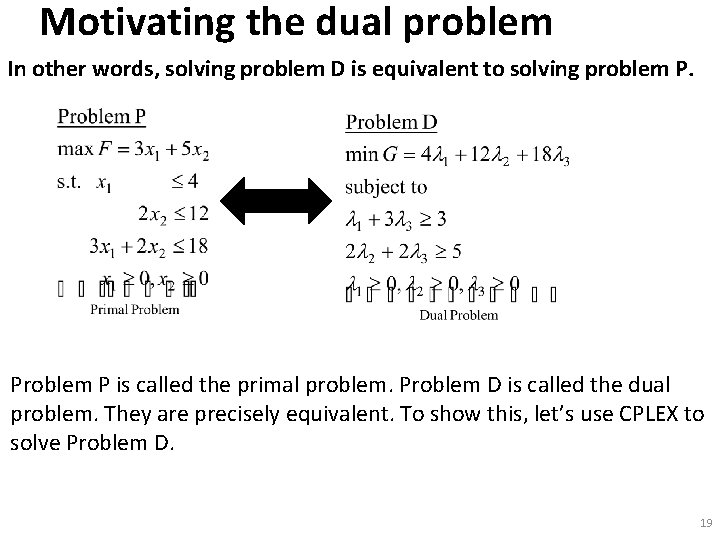
Motivating the dual problem Consider our now very familiar example problem (call it P): P Let’s express linear combinations of multiples of the constraints, where the constraint multipliers are denoted λi on the ith constraint. We assume that λi≥ 0 to avoid having to change the inequality. The composite inequality 12

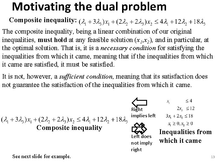
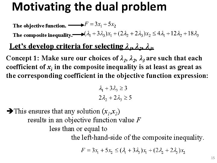
Motivating the dual problem Composite inequality: The composite inequality, being a linear combination of our original inequalities, must hold at any feasible solution (x 1, x 2), and in particular, at the optimal solution. That is, it is a necessary condition for satisfying the inequalities from which it came, meaning that if the inequalities from which it came are satisfied, it must be satisfied. It is not, however, a sufficient condition, meaning that its satisfaction does not guarantee the satisfaction of the inequalities from which it came. Right implies left Composite inequality Left does not imply right See next slide for example. Inequalities from which it came 13

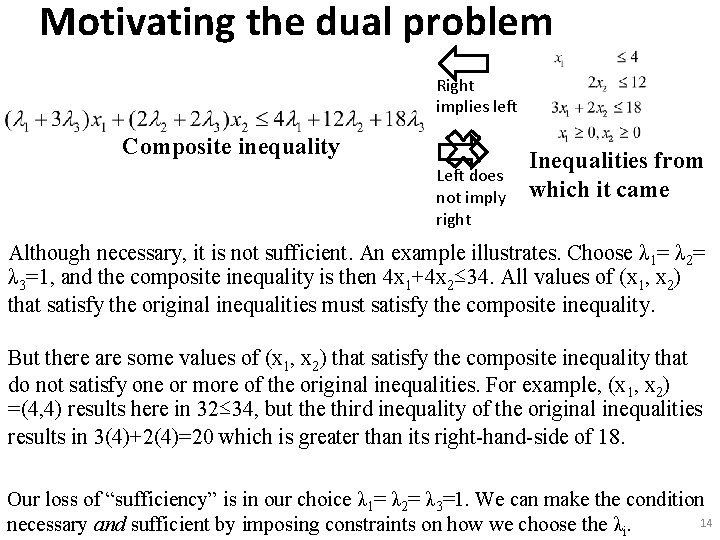
Motivating the dual problem Right implies left Composite inequality Left does not imply right Inequalities from which it came Although necessary, it is not sufficient. An example illustrates. Choose λ 1= λ 2= λ 3=1, and the composite inequality is then 4 x 1+4 x 2≤ 34. All values of (x 1, x 2) that satisfy the original inequalities must satisfy the composite inequality. But there are some values of (x 1, x 2) that satisfy the composite inequality that do not satisfy one or more of the original inequalities. For example, (x 1, x 2) =(4, 4) results here in 32≤ 34, but the third inequality of the original inequalities results in 3(4)+2(4)=20 which is greater than its right-hand-side of 18. Our loss of “sufficiency” is in our choice λ 1= λ 2= λ 3=1. We can make the condition 14 necessary and sufficient by imposing constraints on how we choose the λi.

Motivating the dual problem The objective function. The composite inequality. Let’s develop criteria for selecting λ 1, λ 2, λ 3. Concept 1: Make sure our choices of λ 1, λ 2, λ 3 are such that each coefficient of xi in the composite inequality is at least as great as the corresponding coefficient in the objective function expression: This ensures that any solution (x 1, x 2) results in an objective function value F less than or equal to the left-hand-side of the composite inequality. 15

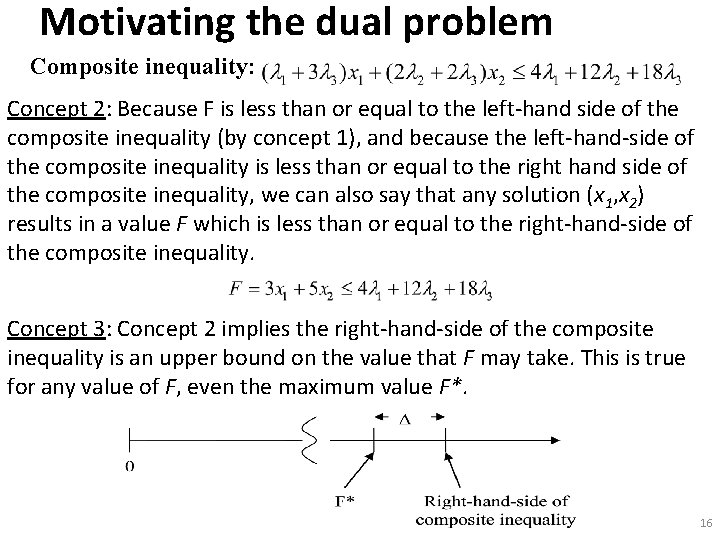
Motivating the dual problem Composite inequality: Concept 2: Because F is less than or equal to the left-hand side of the composite inequality (by concept 1), and because the left-hand-side of the composite inequality is less than or equal to the right hand side of the composite inequality, we can also say that any solution (x 1, x 2) results in a value F which is less than or equal to the right-hand-side of the composite inequality. Concept 3: Concept 2 implies the right-hand-side of the composite inequality is an upper bound on the value that F may take. This is true for any value of F, even the maximum value F*. 16

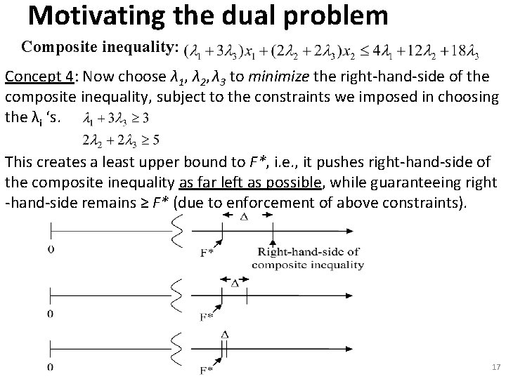
Motivating the dual problem Composite inequality: Concept 4: Now choose λ 1, λ 2, λ 3 to minimize the right-hand-side of the composite inequality, subject to the constraints we imposed in choosing the λi ‘s. This creates a least upper bound to F*, i. e. , it pushes right-hand-side of the composite inequality as far left as possible, while guaranteeing right -hand-side remains ≥ F* (due to enforcement of above constraints). 17

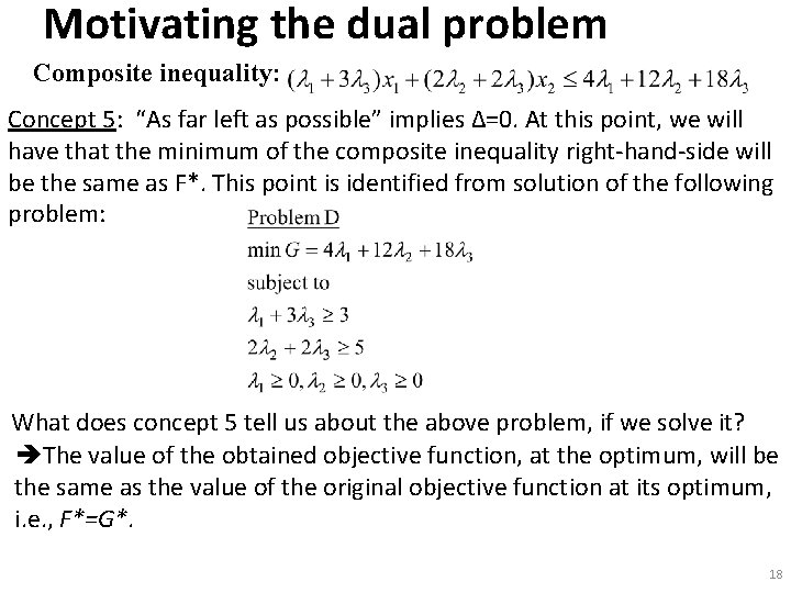
Motivating the dual problem Composite inequality: Concept 5: “As far left as possible” implies Δ=0. At this point, we will have that the minimum of the composite inequality right-hand-side will be the same as F*. This point is identified from solution of the following problem: What does concept 5 tell us about the above problem, if we solve it? The value of the obtained objective function, at the optimum, will be the same as the value of the original objective function at its optimum, i. e. , F*=G*. 18

Motivating the dual problem In other words, solving problem D is equivalent to solving problem P. Problem P is called the primal problem. Problem D is called the dual problem. They are precisely equivalent. To show this, let’s use CPLEX to solve Problem D. 19

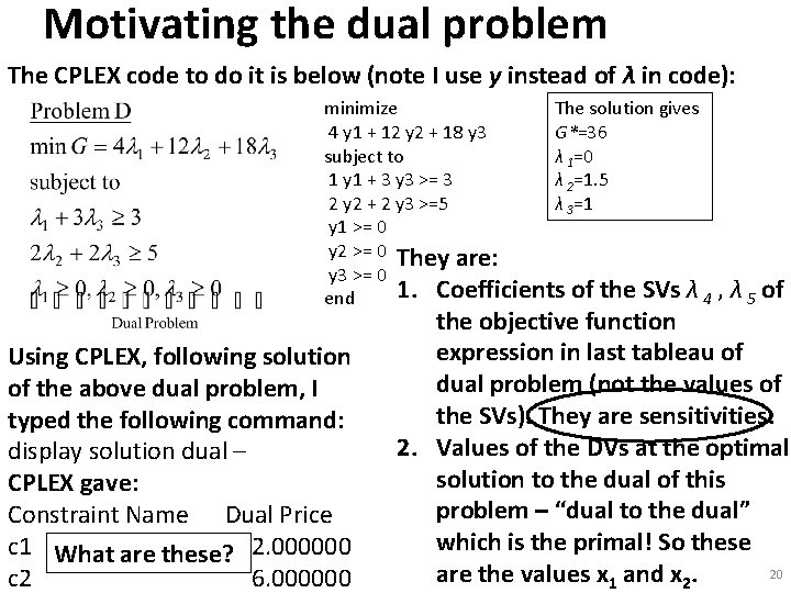
Motivating the dual problem The CPLEX code to do it is below (note I use y instead of λ in code): minimize The solution gives 4 y 1 + 12 y 2 + 18 y 3 G*=36 subject to λ 1=0 1 y 1 + 3 y 3 >= 3 λ 2=1. 5 2 y 2 + 2 y 3 >=5 λ 3=1 y 1 >= 0 y 2 >= 0 They are: y 3 >= 0 1. Coefficients of the SVs λ 4 , λ 5 end Using CPLEX, following solution of the above dual problem, I typed the following command: display solution dual – CPLEX gave: Constraint Name Dual Price c 1 What are these? 2. 000000 c 2 6. 000000 of the objective function expression in last tableau of dual problem (not the values of the SVs). They are sensitivities. 2. Values of the DVs at the optimal solution to the dual of this problem – “dual to the dual” which is the primal! So these 20 are the values x 1 and x 2.

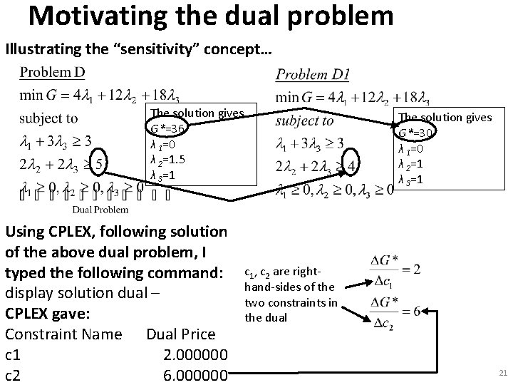
Motivating the dual problem Illustrating the “sensitivity” concept… The solution gives G*=36 λ 1=0 λ 2=1. 5 λ 3=1 Using CPLEX, following solution of the above dual problem, I typed the following command: display solution dual – CPLEX gave: Constraint Name Dual Price c 1 2. 000000 c 2 6. 000000 The solution gives G*=30 λ 1=0 λ 2=1 λ 3=1 c 1, c 2 are righthand-sides of the two constraints in the dual 21

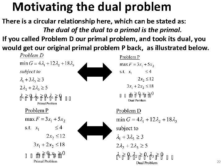
Motivating the dual problem There is a circular relationship here, which can be stated as: The dual of the dual to a primal is the primal. If you called Problem D our primal problem, and took its dual, you would get our original primal problem P back, as illustrated below. 22

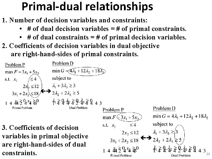
Primal-dual relationships 1. Number of decision variables and constraints: • # of dual decision variables = # of primal constraints. • # of dual constraints = # of primal decision variables. 2. Coefficients of decision variables in dual objective are right-hand-sides of primal constraints. 3. Coefficients of decision variables in primal objective are right-hand-sides of dual constraints. 23

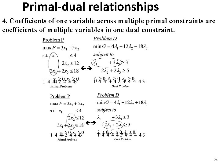
Primal-dual relationships 4. Coefficients of one variable across multiple primal constraints are coefficients of multiple variables in one dual constraint. 24

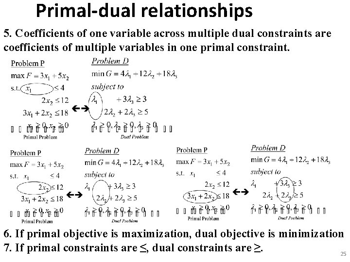
Primal-dual relationships 5. Coefficients of one variable across multiple dual constraints are coefficients of multiple variables in one primal constraint. 6. If primal objective is maximization, dual objective is minimization 7. If primal constraints are ≤, dual constraints are ≥. 25

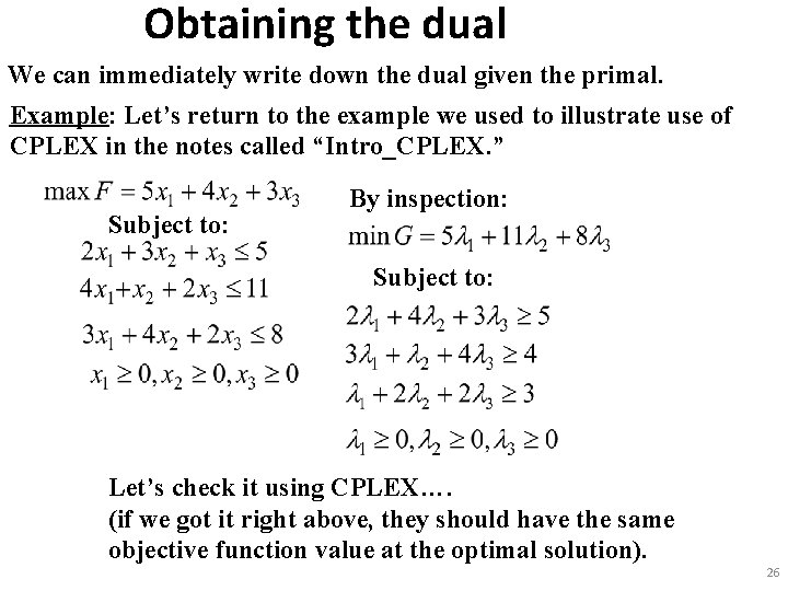
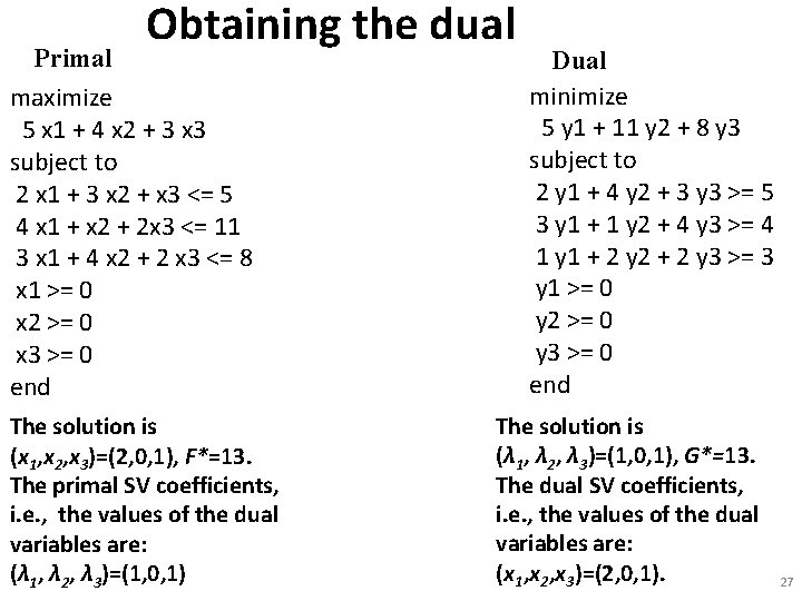
Obtaining the dual We can immediately write down the dual given the primal. Example: Let’s return to the example we used to illustrate use of CPLEX in the notes called “Intro_CPLEX. ” Subject to: By inspection: Subject to: Let’s check it using CPLEX…. (if we got it right above, they should have the same objective function value at the optimal solution). 26

Obtaining the dual Primal maximize 5 x 1 + 4 x 2 + 3 x 3 subject to 2 x 1 + 3 x 2 + x 3 <= 5 4 x 1 + x 2 + 2 x 3 <= 11 3 x 1 + 4 x 2 + 2 x 3 <= 8 x 1 >= 0 x 2 >= 0 x 3 >= 0 end The solution is (x 1, x 2, x 3)=(2, 0, 1), F*=13. The primal SV coefficients, i. e. , the values of the dual variables are: (λ 1, λ 2, λ 3)=(1, 0, 1) Dual minimize 5 y 1 + 11 y 2 + 8 y 3 subject to 2 y 1 + 4 y 2 + 3 y 3 >= 5 3 y 1 + 1 y 2 + 4 y 3 >= 4 1 y 1 + 2 y 2 + 2 y 3 >= 3 y 1 >= 0 y 2 >= 0 y 3 >= 0 end The solution is (λ 1, λ 2, λ 3)=(1, 0, 1), G*=13. The dual SV coefficients, i. e. , the values of the dual variables are: (x 1, x 2, x 3)=(2, 0, 1). 27

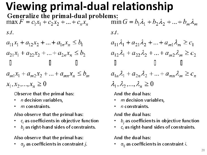
Viewing primal-dual relationship Generalize the primal-dual problems: Observe that the primal has: • n decision variables, • m constraints. And the dual has: • m decision variables, • n constraints. Also observe that the primal has: • ci as coefficients in objective function • bj as right-hand sides of constraints. And the dual has: • bj as coefficients in objective function • ci as right-hand sides of constraints. Also observe that the primal has: • aji as coefficients in constraint j. And the dual has: • aij as coefficients in constraint i. 28

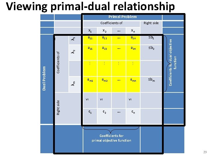
Viewing primal-dual relationship Primal Problem Coefficients of λ 2 λm Coefficients of Dual Problem Right side x 1 x 2 … xn a 11 a 12 … a 1 n ≤b 1 a 22 … a 2 n ≤b 2 ⁞ ⁞ am 1 am 2 … amn c 1 c 2 ≤bm ≤ ≤ ≤ Right side Coefficients for dual objective function λ 1 … Coefficients for primal objective function cn 29

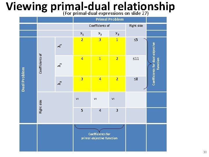
Viewing primal-dual relationship (For primal-dual expressions on slide 27) Primal Problem Coefficients of Right side x 1 x 2 x 3 2 3 1 ≤ 5 4 1 2 ≤ 11 3 4 2 ≤ 8 λ 2 ≤ ≤ ≤ λ 3 Coefficients of Right side Dual Problem 5 Coefficients for dual objective function λ 1 4 3 Coefficients for primal objective function 30

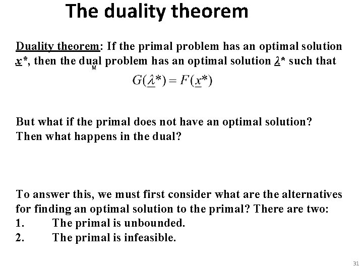
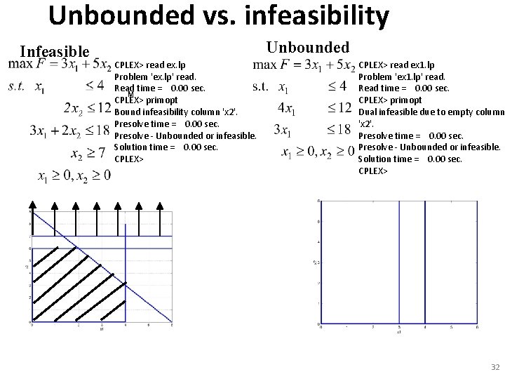
The duality theorem Duality theorem: If the primal problem has an optimal solution x*, then the dual problem has an optimal solution λ* such that But what if the primal does not have an optimal solution? Then what happens in the dual? To answer this, we must first consider what are the alternatives for finding an optimal solution to the primal? There are two: 1. The primal is unbounded. 2. The primal is infeasible. 31

Unbounded vs. infeasibility Infeasible Unbounded CPLEX> read ex. lp Problem 'ex. lp' read. Read time = 0. 00 sec. CPLEX> primopt Bound infeasibility column 'x 2'. Presolve time = 0. 00 sec. Presolve - Unbounded or infeasible. Solution time = 0. 00 sec. CPLEX> read ex 1. lp Problem 'ex 1. lp' read. Read time = 0. 00 sec. CPLEX> primopt Dual infeasible due to empty column 'x 2'. Presolve time = 0. 00 sec. Presolve - Unbounded or infeasible. Solution time = 0. 00 sec. CPLEX> 32

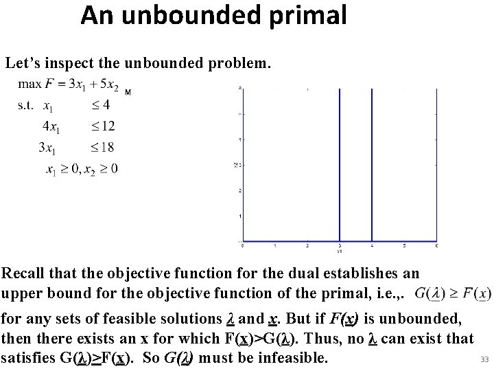
An unbounded primal Let’s inspect the unbounded problem. Recall that the objective function for the dual establishes an upper bound for the objective function of the primal, i. e. , . for any sets of feasible solutions λ and x. But if F(x) is unbounded, then there exists an x for which F(x)>G(λ). Thus, no λ can exist that satisfies G(λ)>F(x). So G(λ) must be infeasible. 33

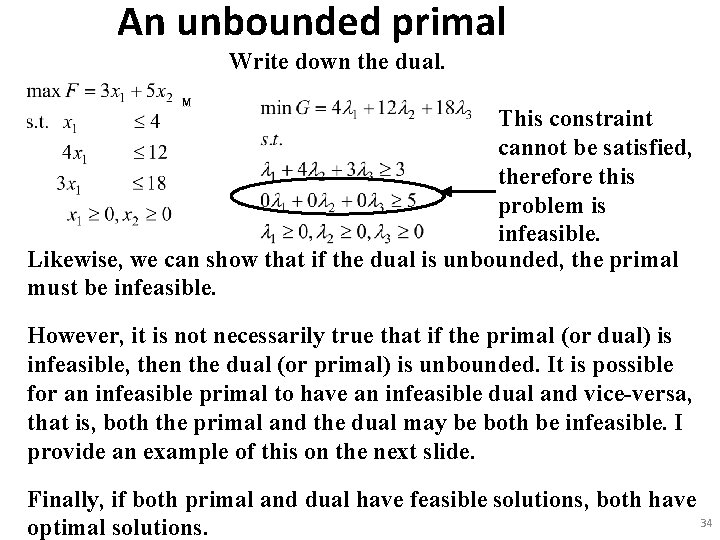
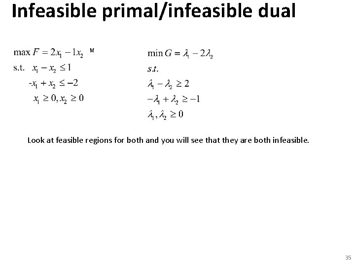
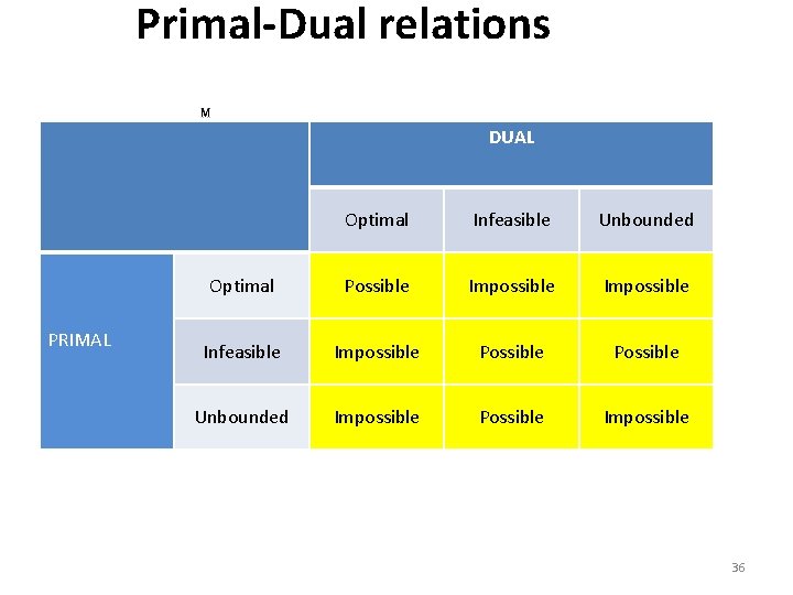
An unbounded primal Write down the dual. This constraint cannot be satisfied, therefore this problem is infeasible. Likewise, we can show that if the dual is unbounded, the primal must be infeasible. However, it is not necessarily true that if the primal (or dual) is infeasible, then the dual (or primal) is unbounded. It is possible for an infeasible primal to have an infeasible dual and vice-versa, that is, both the primal and the dual may be both be infeasible. I provide an example of this on the next slide. Finally, if both primal and dual have feasible solutions, both have 34 optimal solutions.

Infeasible primal/infeasible dual Look at feasible regions for both and you will see that they are both infeasible. 35

Primal-Dual relations DUAL PRIMAL Optimal Infeasible Unbounded Optimal Possible Impossible Infeasible Impossible Possible Unbounded Impossible Possible Impossible 36

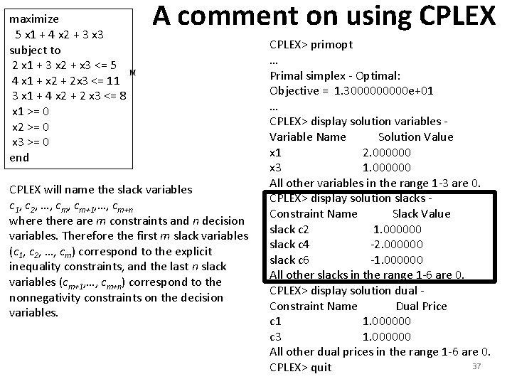
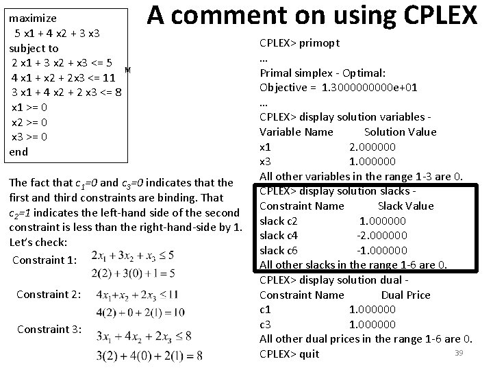
maximize 5 x 1 + 4 x 2 + 3 x 3 subject to 2 x 1 + 3 x 2 + x 3 <= 5 4 x 1 + x 2 + 2 x 3 <= 11 3 x 1 + 4 x 2 + 2 x 3 <= 8 x 1 >= 0 x 2 >= 0 x 3 >= 0 end A comment on using CPLEX will name the slack variables c 1, c 2, …, cm+1, …, cm+n where there are m constraints and n decision variables. Therefore the first m slack variables (c 1, c 2, …, cm) correspond to the explicit inequality constraints, and the last n slack variables (cm+1, …, cm+n) correspond to the nonnegativity constraints on the decision variables. CPLEX> primopt … Primal simplex - Optimal: Objective = 1. 300000 e+01 … CPLEX> display solution variables Variable Name Solution Value x 1 2. 000000 x 3 1. 000000 All other variables in the range 1 -3 are 0. CPLEX> display solution slacks Constraint Name Slack Value slack c 2 1. 000000 slack c 4 -2. 000000 slack c 6 -1. 000000 All other slacks in the range 1 -6 are 0. CPLEX> display solution dual Constraint Name Dual Price c 1 1. 000000 c 3 1. 000000 All other dual prices in the range 1 -6 are 0. 37 CPLEX> quit

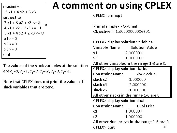
maximize 5 x 1 + 4 x 2 + 3 x 3 subject to 2 x 1 + 3 x 2 + x 3 <= 5 4 x 1 + x 2 + 2 x 3 <= 11 3 x 1 + 4 x 2 + 2 x 3 <= 8 x 1 >= 0 x 2 >= 0 x 3 >= 0 end A comment on using CPLEX> primopt … Primal simplex - Optimal: Objective = 1. 300000 e+01 … CPLEX> display solution variables Variable Name Solution Value x 1 2. 000000 x 3 1. 000000 All other variables in the range 1 -3 are 0. The values of the slack variables at the solution CPLEX> display solution slacks are c 1=0, c 2=1, c 3=0, c 4=-2, c 5=0, c 6=-1. Constraint Name Slack Value slack c 2 1. 000000 Note that CPLEX does not print the values of slack c 4 -2. 000000 slack variables that are zero. slack c 6 -1. 000000 All other slacks in the range 1 -6 are 0. CPLEX> display solution dual Constraint Name Dual Price c 1 1. 000000 c 3 1. 000000 All other dual prices in the range 1 -6 are 0. 38 CPLEX> quit

maximize 5 x 1 + 4 x 2 + 3 x 3 subject to 2 x 1 + 3 x 2 + x 3 <= 5 4 x 1 + x 2 + 2 x 3 <= 11 3 x 1 + 4 x 2 + 2 x 3 <= 8 x 1 >= 0 x 2 >= 0 x 3 >= 0 end A comment on using CPLEX The fact that c 1=0 and c 3=0 indicates that the first and third constraints are binding. That c 2=1 indicates the left-hand side of the second constraint is less than the right-hand-side by 1. Let’s check: Constraint 1: Constraint 2: Constraint 3: CPLEX> primopt … Primal simplex - Optimal: Objective = 1. 300000 e+01 … CPLEX> display solution variables Variable Name Solution Value x 1 2. 000000 x 3 1. 000000 All other variables in the range 1 -3 are 0. CPLEX> display solution slacks Constraint Name Slack Value slack c 2 1. 000000 slack c 4 -2. 000000 slack c 6 -1. 000000 All other slacks in the range 1 -6 are 0. CPLEX> display solution dual Constraint Name Dual Price c 1 1. 000000 c 3 1. 000000 All other dual prices in the range 1 -6 are 0. 39 CPLEX> quit

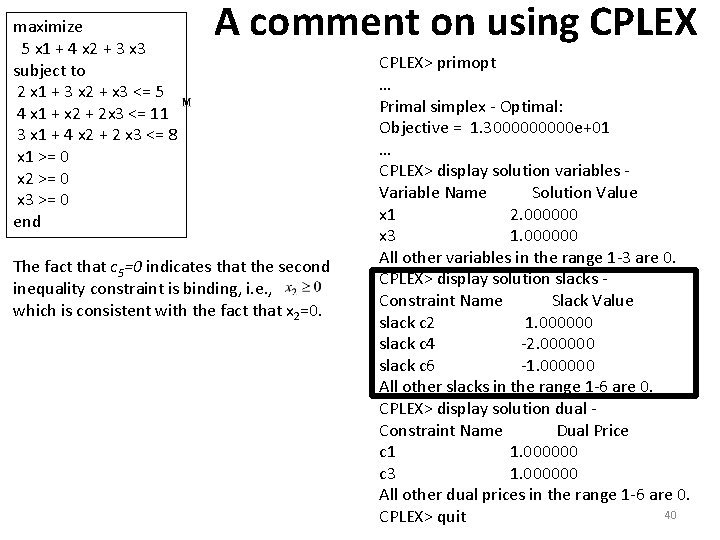
maximize 5 x 1 + 4 x 2 + 3 x 3 subject to 2 x 1 + 3 x 2 + x 3 <= 5 4 x 1 + x 2 + 2 x 3 <= 11 3 x 1 + 4 x 2 + 2 x 3 <= 8 x 1 >= 0 x 2 >= 0 x 3 >= 0 end A comment on using CPLEX The fact that c 5=0 indicates that the second inequality constraint is binding, i. e. , which is consistent with the fact that x 2=0. CPLEX> primopt … Primal simplex - Optimal: Objective = 1. 300000 e+01 … CPLEX> display solution variables Variable Name Solution Value x 1 2. 000000 x 3 1. 000000 All other variables in the range 1 -3 are 0. CPLEX> display solution slacks Constraint Name Slack Value slack c 2 1. 000000 slack c 4 -2. 000000 slack c 6 -1. 000000 All other slacks in the range 1 -6 are 0. CPLEX> display solution dual Constraint Name Dual Price c 1 1. 000000 c 3 1. 000000 All other dual prices in the range 1 -6 are 0. 40 CPLEX> quit

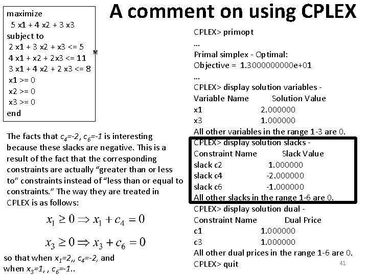
maximize 5 x 1 + 4 x 2 + 3 x 3 subject to 2 x 1 + 3 x 2 + x 3 <= 5 4 x 1 + x 2 + 2 x 3 <= 11 3 x 1 + 4 x 2 + 2 x 3 <= 8 x 1 >= 0 x 2 >= 0 x 3 >= 0 end A comment on using CPLEX> primopt … Primal simplex - Optimal: Objective = 1. 300000 e+01 … CPLEX> display solution variables Variable Name Solution Value x 1 2. 000000 x 3 1. 000000 All other variables in the range 1 -3 are 0. The facts that c 4=-2, c 6=-1 is interesting CPLEX> display solution slacks because these slacks are negative. This is a Constraint Name Slack Value result of the fact that the corresponding slack c 2 1. 000000 constraints are actually “greater than or less slack c 4 -2. 000000 to” constraints instead of “less than or equal to slack c 6 -1. 000000 constraints. ” The way they are treated in All other slacks in the range 1 -6 are 0. CPLEX is as follows: CPLEX> display solution dual Constraint Name Dual Price c 1 1. 000000 c 3 1. 000000 All other dual prices in the range 1 -6 are 0. so that when x 1=2, , c 4=-2, and 41 CPLEX> quit when x 3=1, , c 6=-1. .

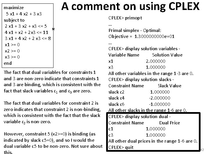
maximize 5 x 1 + 4 x 2 + 3 x 3 subject to 2 x 1 + 3 x 2 + x 3 <= 5 4 x 1 + x 2 + 2 x 3 <= 11 3 x 1 + 4 x 2 + 2 x 3 <= 8 x 1 >= 0 x 2 >= 0 x 3 >= 0 end A comment on using CPLEX> primopt … Primal simplex - Optimal: Objective = 1. 300000 e+01 … CPLEX> display solution variables Variable Name Solution Value x 1 2. 000000 x 3 1. 000000 The fact that dual variables for constraints 1 All other variables in the range 1 -3 are 0. and 3 are non-zero indicate that constraints 1 CPLEX> display solution slacks and 3 are binding, which is consistent with the Constraint Name Slack Value fact that slack variables c 1 and c 3 are zero. slack c 2 1. 000000 slack c 4 -2. 000000 The fact that dual variables for constraint 2 is slack c 6 -1. 000000 zero indicates that constraint 2 is non-binding, All other slacks in the range 1 -6 are 0. which is consistent with the fact that the slack CPLEX> display solution dual variable c 2 is non-zero. Constraint Name Dual Price c 1 1. 000000 However, constraint 5 (x 2>=0) is binding (as c 3 1. 000000 indicated by slack c 5=0), and so I would the All other dual prices in the range 1 -6 are 0. dual variable c 5 to be non-zero. Not sure about CPLEX> quit this. 42