EEEcon 458 Integer Programming J Mc Calley 1

EE/Econ 458 Integer Programming J. Mc. Calley 1

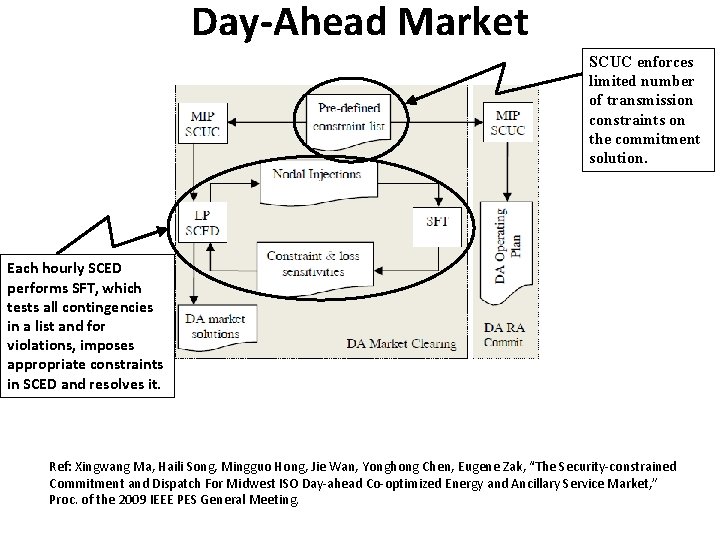
Day-Ahead Market SCUC enforces limited number of transmission constraints on the commitment solution. Each hourly SCED performs SFT, which tests all contingencies in a list and for violations, imposes appropriate constraints in SCED and resolves it. Ref: Xingwang Ma, Haili Song, Mingguo Hong, Jie Wan, Yonghong Chen, Eugene Zak, “The Security-constrained Commitment and Dispatch For Midwest ISO Day-ahead Co-optimized Energy and Ancillary Service Market, ” Proc. of the 2009 IEEE PES General Meeting.

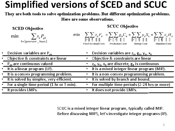
Simplified versions of SCED and SCUC They are both tools to solve optimization problems. But different optimization problems. Here are some observations. SCUC Objective SCED Objective • • Decision variables are Pgk Objective & constraints are linear Pgk are continuous valued It is a linear program (LP). It is a convex programming problem. It is solved by simplex, very efficient. For a single time period (1 hr or 5 min). It provides LMPs. • • Decision variables are zit, git, yit, xit Objective & constraints are linear zit, yit, xit are discrete, git is continuous It is a mixed integer linear program (MIP). It is a non-convex programming problem. It is solved by branch and bound. For multiple time periods (2 -24 hrs or more) It does not provide LMPs. SCUC is a mixed integer linear program, typically called MIP. Before discussing MIPS, let’s investigate integer programs (IP). 3

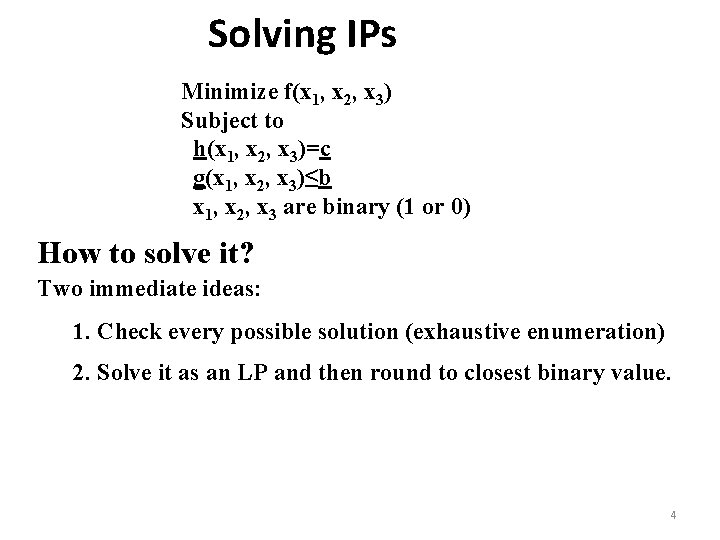
Solving IPs Minimize f(x 1, x 2, x 3) Subject to h(x 1, x 2, x 3)=c g(x 1, x 2, x 3)≤b x 1, x 2, x 3 are binary (1 or 0) How to solve it? Two immediate ideas: 1. Check every possible solution (exhaustive enumeration) 2. Solve it as an LP and then round to closest binary value. 4

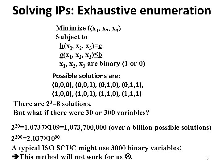
Solving IPs: Exhaustive enumeration Minimize f(x 1, x 2, x 3) Subject to h(x 1, x 2, x 3)=c g(x 1, x 2, x 3)≤b x 1, x 2, x 3 are binary (1 or 0) Possible solutions are: (0, 0, 0), (0, 0, 1), (0, 1, 0), (0, 1, 1), (1, 0, 0), (1, 0, 1), (1, 1, 0), (1, 1, 1) There are 23=8 solutions. But what if there were 30 or 300 variables? 230=1. 0737× 109=1, 073, 700, 000 (over a billion possible solutions) 2300=2. 037× 1090 A typical ISO SCUC might use 3000 binary variables! This method will not work for us . 5

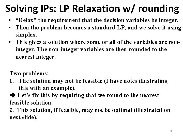
Solving IPs: LP Relaxation w/ rounding • “Relax” the requirement that the decision variables be integer. • Then the problem becomes a standard LP, and we solve it using simplex. • This gives a solution where some or all of the variables are noninteger. The non-integer variables are then rounded to the nearest integer. Two problems: 1. The solution may not be feasible (I have notes illustrating this with an example). Let’s fix this by requiring that we round to the nearest feasible solution. 2. This solution, if feasible, may not be optimal (illustrated on next slide). 6

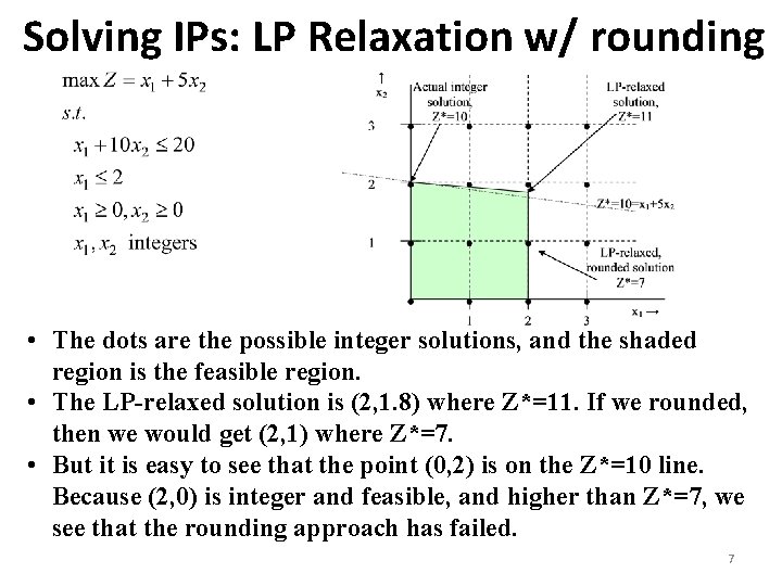
Solving IPs: LP Relaxation w/ rounding • The dots are the possible integer solutions, and the shaded region is the feasible region. • The LP-relaxed solution is (2, 1. 8) where Z*=11. If we rounded, then we would get (2, 1) where Z*=7. • But it is easy to see that the point (0, 2) is on the Z*=10 line. Because (2, 0) is integer and feasible, and higher than Z*=7, we see that the rounding approach has failed. 7

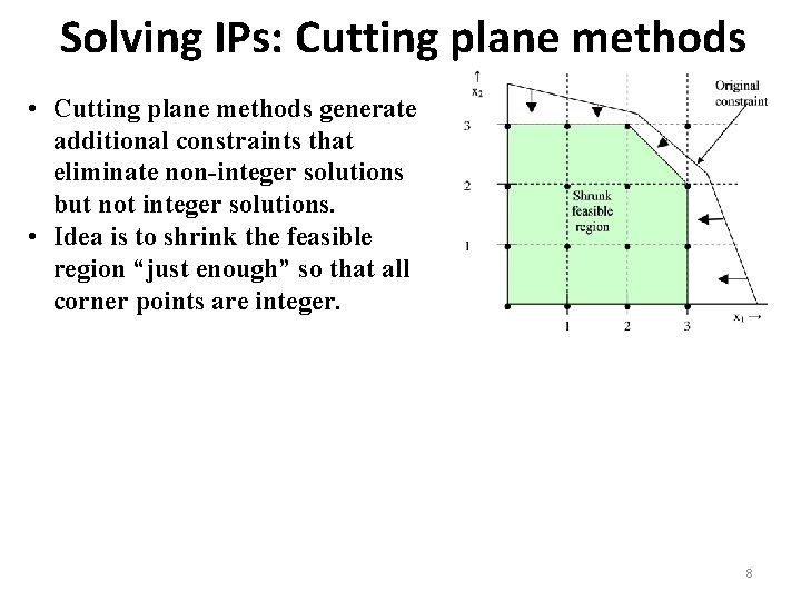
Solving IPs: Cutting plane methods • Cutting plane methods generate additional constraints that eliminate non-integer solutions but not integer solutions. • Idea is to shrink the feasible region “just enough” so that all corner points are integer. 8

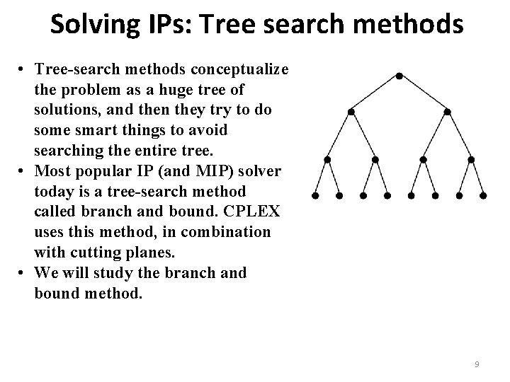
Solving IPs: Tree search methods • Tree-search methods conceptualize the problem as a huge tree of solutions, and then they try to do some smart things to avoid searching the entire tree. • Most popular IP (and MIP) solver today is a tree-search method called branch and bound. CPLEX uses this method, in combination with cutting planes. • We will study the branch and bound method. 9

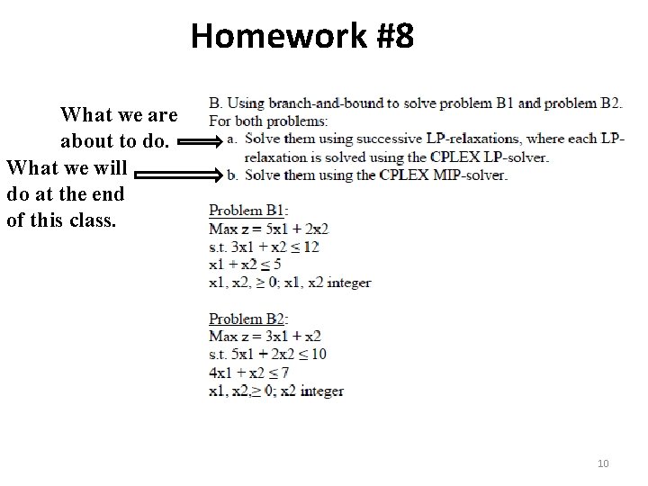
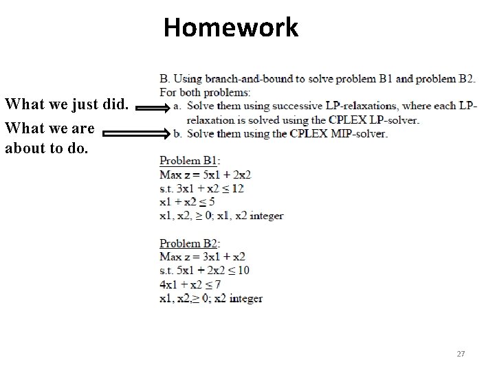
Homework #8 What we are about to do. What we will do at the end of this class. 10

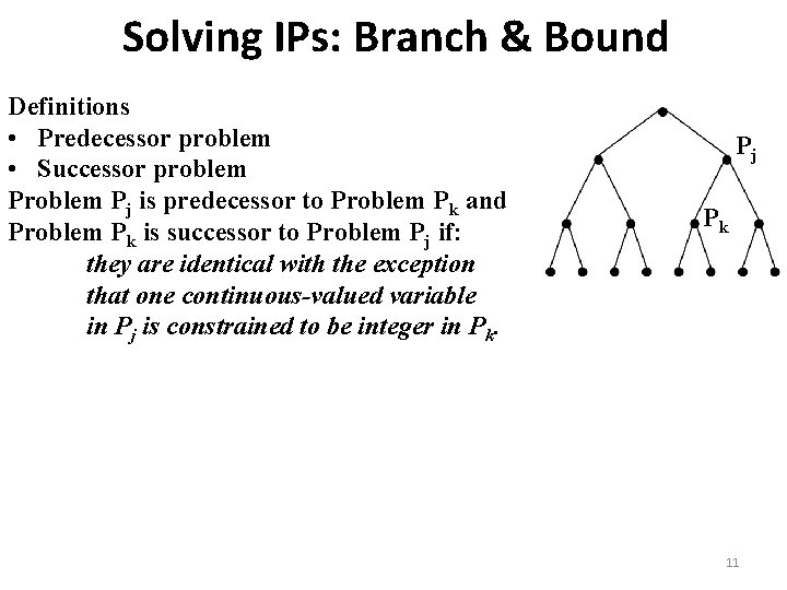
Solving IPs: Branch & Bound Definitions • Predecessor problem • Successor problem Pj is predecessor to Problem Pk and Problem Pk is successor to Problem Pj if: they are identical with the exception that one continuous-valued variable in Pj is constrained to be integer in Pk. Pj Pk 11

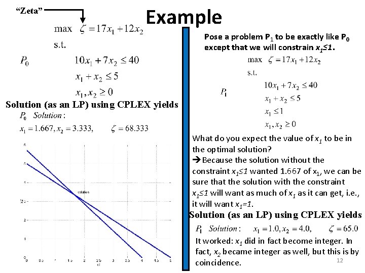
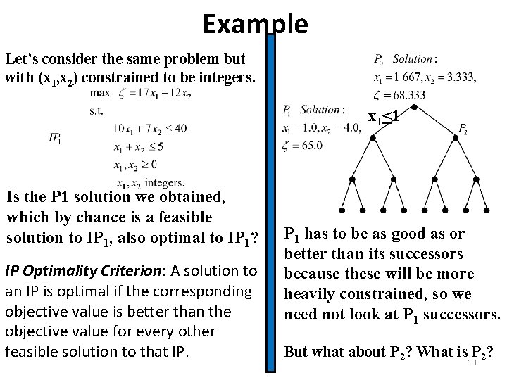
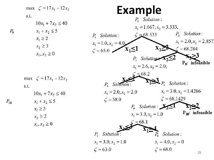
“Zeta” Example Pose a problem P 1 to be exactly like P 0 except that we will constrain x 1≤ 1. Solution (as an LP) using CPLEX yields What do you expect the value of x 1 to be in the optimal solution? Because the solution without the constraint x 1≤ 1 wanted 1. 667 of x 1, we can be sure that the solution with the constraint x 1≤ 1 will want as much of x 1 as it can get, i. e. , it will want x 1=1. Solution (as an LP) using CPLEX yields It worked: x 1 did in fact become integer. In fact, x 2 became integer as well, but this is by 12 coincidence.

Example Let’s consider the same problem but with (x 1, x 2) constrained to be integers. x 1<1 Is the P 1 solution we obtained, which by chance is a feasible solution to IP 1, also optimal to IP 1? IP Optimality Criterion: A solution to an IP is optimal if the corresponding objective value is better than the objective value for every other feasible solution to that IP. P 1 has to be as good as or better than its successors because these will be more heavily constrained, so we need not look at P 1 successors. But what about P 2? What is P 2? 13

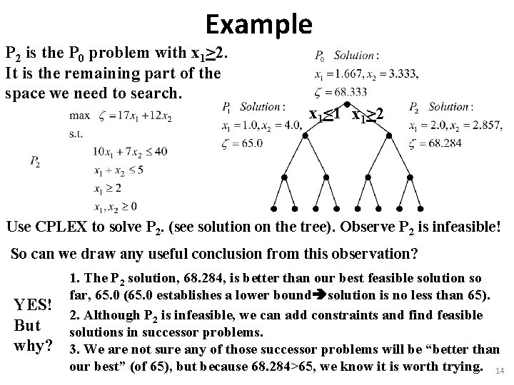
Example P 2 is the P 0 problem with x 1>2. It is the remaining part of the space we need to search. x 1<1 x 1>2 Use CPLEX to solve P 2. (see solution on the tree). Observe P 2 is infeasible! So can we draw any useful conclusion from this observation? YES! But why? 1. The P 2 solution, 68. 284, is better than our best feasible solution so far, 65. 0 (65. 0 establishes a lower bound solution is no less than 65). 2. Although P 2 is infeasible, we can add constraints and find feasible solutions in successor problems. 3. We are not sure any of those successor problems will be “better than our best” (of 65), but because 68. 284>65, we know it is worth trying. 14

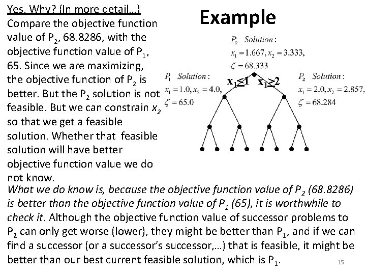
Yes, Why? (In more detail…) Compare the objective function value of P 2, 68. 8286, with the objective function value of P 1, 65. Since we are maximizing, the objective function of P 2 is x 1<1 x 1>2 better. But the P 2 solution is not feasible. But we can constrain x 2 so that we get a feasible solution. Whether that feasible solution will have better objective function value we do not know. What we do know is, because the objective function value of P 2 (68. 8286) is better than the objective function value of P 1 (65), it is worthwhile to check it. Although the objective function value of successor problems to P 2 can only get worse (lower), they might be better than P 1, and if we can find a successor (or a successor’s successor, …) that is feasible, it might be better than our best current feasible solution, which is P 1. 15 Example

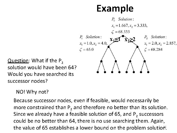
Example x 1<1 x 1>2 Question: What if the P 2 solution would have been 64? Would you have searched its successor nodes? NO! Why not? Because successor nodes, even if feasible, would necessarily be more constrained than P 2 and therefore no better than its solution. Since we already have a feasible solution of 65, and P 2 successors could be no better than 64, there is no use searching them. Again, 16 the value of 65 establishes a lower bound on the problem solution.

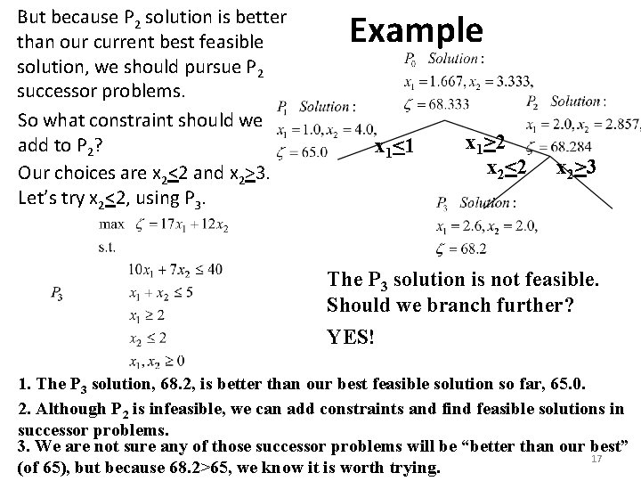
But because P 2 solution is better than our current best feasible solution, we should pursue P 2 successor problems. So what constraint should we add to P 2? Our choices are x 2<2 and x 2>3. Let’s try x 2<2, using P 3. Example x 1<1 x 1>2 x 2<2 x 2>3 The P 3 solution is not feasible. Should we branch further? YES! 1. The P 3 solution, 68. 2, is better than our best feasible solution so far, 65. 0. 2. Although P 2 is infeasible, we can add constraints and find feasible solutions in successor problems. 3. We are not sure any of those successor problems will be “better than our best” 17 (of 65), but because 68. 2>65, we know it is worth trying.

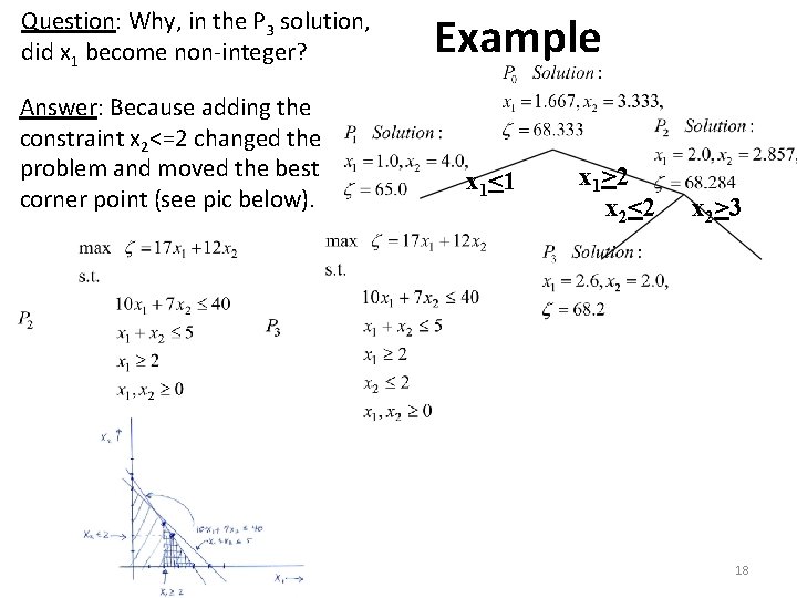
Question: Why, in the P 3 solution, did x 1 become non-integer? Answer: Because adding the constraint x 2<=2 changed the problem and moved the best corner point (see pic below). Example x 1<1 x 1>2 x 2<2 x 2>3 18

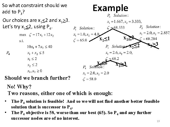
So what constraint should we add to P 3? Example Our choices are x 1<2 and x 1>3. Let’s try x 1<2, using P 4. x 1<1 x 1<2 x 1>2 x 2<2 x 2>3 x 1>3 Should we branch further? No! Why? Two reasons, either one of which is enough: • The P 4 solution is feasible! And so we will not find another better feasible solution that is successor to P 4. • The P 4 objective is 58, worse than our best (65). So P 4 and any further successor nodes are of no interest. 19

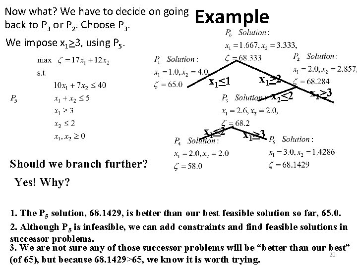
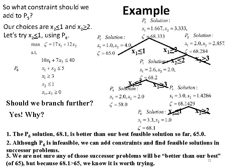
Now what? We have to decide on going back to P 3 or P 2. Choose P 3. Example We impose x 1>3, using P 5. x 1<1 x 1<2 x 1>2 x 2<2 x 2>3 x 1>3 Should we branch further? Yes! Why? 1. The P 5 solution, 68. 1429, is better than our best feasible solution so far, 65. 0. 2. Although P 5 is infeasible, we can add constraints and find feasible solutions in successor problems. 3. We are not sure any of those successor problems will be “better than our best” 20 (of 65), but because 68. 1429>65, we know it is worth trying.

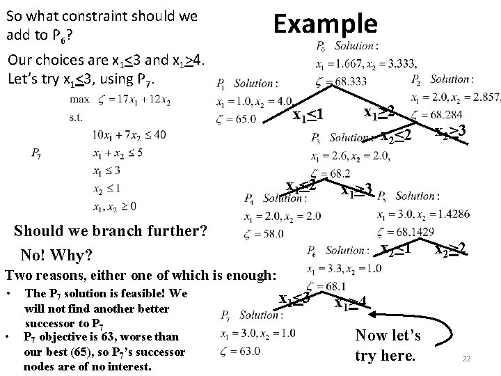
So what constraint should we add to P 5? Example Our choices are x 2<1 and x 2>2. Let’s try x 2<1, using P 6. x 1<1 x 1<2 Should we branch further? Yes! Why? x 1>2 x 2<2 x 2>3 x 1>3 x 2<1 x 2>2 1. The P 6 solution, 68. 1, is better than our best feasible solution so far, 65. 0. 2. Although P 6 is infeasible, we can add constraints and find feasible solutions in successor problems. 3. We are not sure any of those successor problems will be “better than our best” 21 (of 65), but because 68. 1>65, we know it is worth trying.

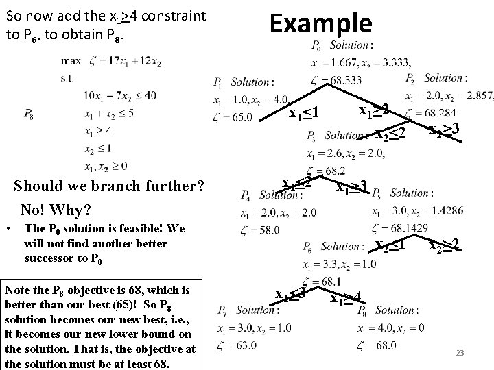
So what constraint should we add to P 6? Example Our choices are x 1<3 and x 1>4. Let’s try x 1<3, using P 7. x 1<1 x 1<2 x 1>2 x 2<2 x 2>3 x 1>3 Should we branch further? No! Why? x 2<1 x 2>2 Two reasons, either one of which is enough: • • The P 7 solution is feasible! We will not find another better successor to P 7 objective is 63, worse than our best (65), so P 7’s successor nodes are of no interest. x 1<3 x 1>4 Now let’s try here. 22

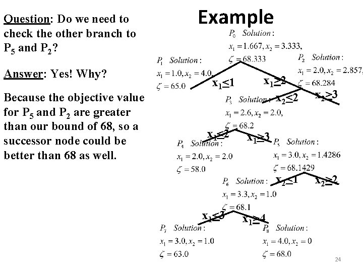
So now add the x 1>4 constraint to P 6, to obtain P 8. Example x 1<1 Should we branch further? No! Why? • x 1<2 x 1>2 x 2<2 x 1>3 The P 8 solution is feasible! We will not find another better successor to P 8 Note the P 8 objective is 68, which is better than our best (65)! So P 8 solution becomes our new best, i. e. , it becomes our new lower bound on the solution. That is, the objective at the solution must be at least 68. x 2<1 x 1<3 x 2>2 x 1>4 23

Question: Do we need to check the other branch to P 5 and P 2? Answer: Yes! Why? Because the objective value for P 5 and P 2 are greater than our bound of 68, so a successor node could be better than 68 as well. Example x 1<1 x 1<2 x 1>2 x 2<2 x 1>3 x 2<1 x 1<3 x 2>2 x 1>4 24

Example x 1<1 x 1<2 x 1>2 x 2<2 P 9: infeasible x 1>3 x 2<1 x 1<3 x 2>2 P 10: infeasible x 1>4 25

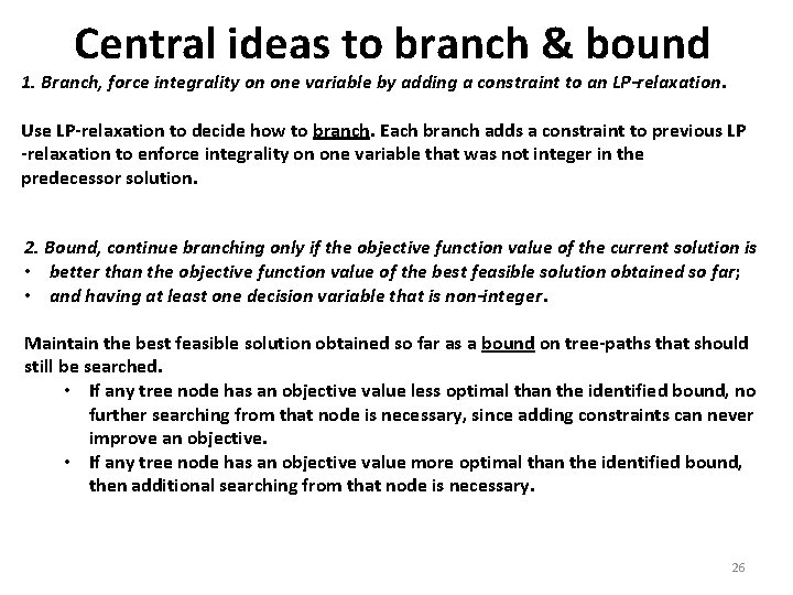
Central ideas to branch & bound 1. Branch, force integrality on one variable by adding a constraint to an LP-relaxation. Use LP-relaxation to decide how to branch. Each branch adds a constraint to previous LP -relaxation to enforce integrality on one variable that was not integer in the predecessor solution. 2. Bound, continue branching only if the objective function value of the current solution is • better than the objective function value of the best feasible solution obtained so far; • and having at least one decision variable that is non-integer. Maintain the best feasible solution obtained so far as a bound on tree-paths that should still be searched. • If any tree node has an objective value less optimal than the identified bound, no further searching from that node is necessary, since adding constraints can never improve an objective. • If any tree node has an objective value more optimal than the identified bound, then additional searching from that node is necessary. 26

Homework What we just did. What we are about to do. 27

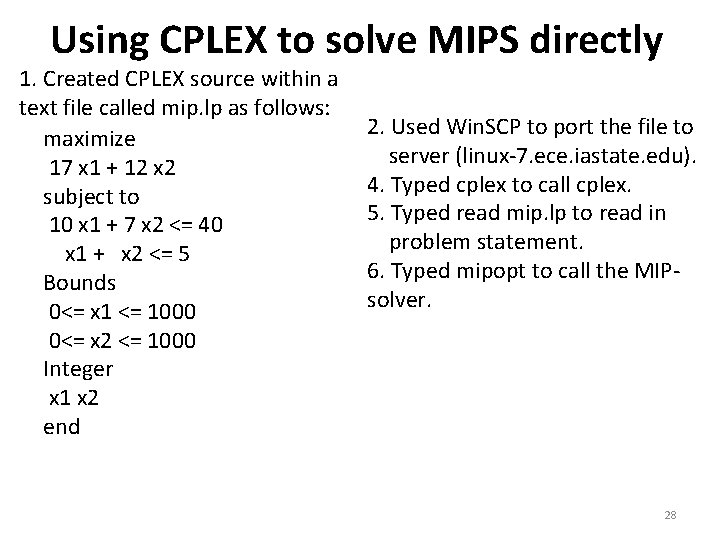
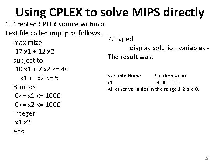
Using CPLEX to solve MIPS directly 1. Created CPLEX source within a text file called mip. lp as follows: maximize 17 x 1 + 12 x 2 subject to 10 x 1 + 7 x 2 <= 40 x 1 + x 2 <= 5 Bounds 0<= x 1 <= 1000 0<= x 2 <= 1000 Integer x 1 x 2 end 2. Used Win. SCP to port the file to server (linux-7. ece. iastate. edu). 4. Typed cplex to call cplex. 5. Typed read mip. lp to read in problem statement. 6. Typed mipopt to call the MIPsolver. 28

Using CPLEX to solve MIPS directly 1. Created CPLEX source within a text file called mip. lp as follows: 7. Typed maximize display solution variables - 17 x 1 + 12 x 2 The result was: subject to 10 x 1 + 7 x 2 <= 40 Variable Name Solution Value x 1 + x 2 <= 5 x 1 4. 000000 Bounds All other variables in the range 1 -2 are 0. 0<= x 1 <= 1000 0<= x 2 <= 1000 Integer x 1 x 2 end 29

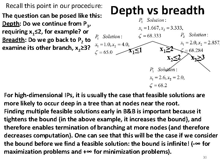
Recall this point in our procedure: The question can be posed like this: Depth: Do we continue from P 3, requiring x 1≤ 2, for example? or Breadth: Do we go back to P 2 to examine its other branch, x 2≥ 3? Depth vs breadth x 1<1 x 1>2 x 2<2 x 2>3 For high-dimensional IPs, it is usually the case that feasible solutions are more likely to occur deep in a tree than at nodes near the root. Finding multiple feasible solutions early in B&B is important because it tightens the bound (in the above example, it increases the bound), and therefore enables termination of branching at more nodes (and therefore decreases computation). One can see that this will be the case if we consider the bound before we find a feasible solution: the bound is infinite! (-∞ for maximization problems and +∞ for minimization problems). 30

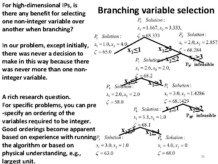
For high-dimensional IPs, is there any benefit for selecting one non-integer variable over another when branching? In our problem, except initially, there was never a decision to make in this way because there was never more than one noninteger variable. A rich research question. For specific problems, you can pre -specify an ordering of the variables required to be integer. Good orderings become apparent based on experience with running the algorithm or based on physical understanding, e. g. , largest unit. Branching variable selection x 1<1 x 1<2 x 1>2 x 2<2 P 9: infeasible x 1>3 x 2<1 x 1<3 x 2>2 P 10: infeasible x 1>4 31

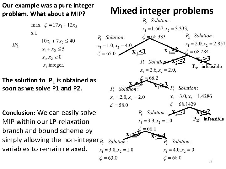
Our example was a pure integer problem. What about a MIP? Mixed integer problems x 1<1 The solution to IP 2 is obtained as soon as we solve P 1 and P 2. x 1<2 x 1>2 x 2<1 x 1<3 P 9: infeasible x 1>3 Conclusion: We can easily solve MIP within our LP-relaxation branch and bound scheme by simply allowing the non-integer variables to remain relaxed. x 2>3 x 2>2 P 10: infeasible x 1>4 32

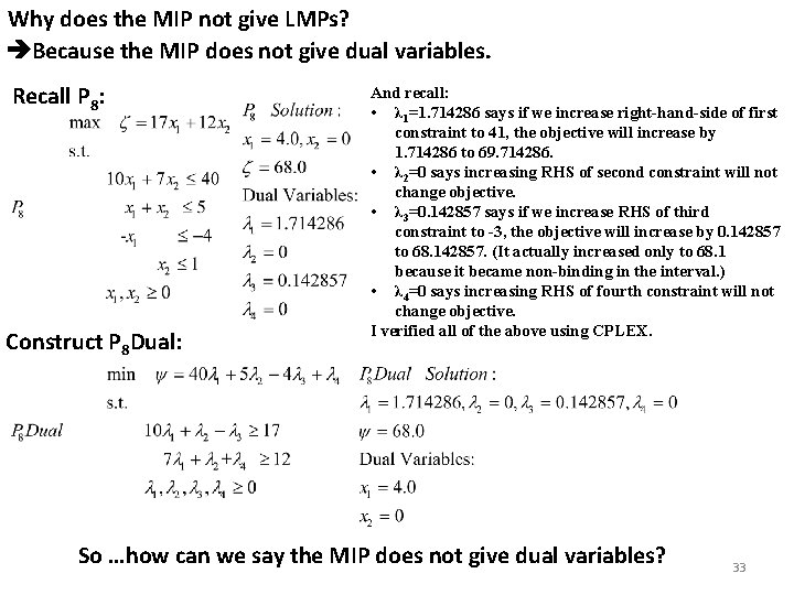
Why does the MIP not give LMPs? Because the MIP does not give dual variables. Recall P 8: Construct P 8 Dual: And recall: • λ 1=1. 714286 says if we increase right-hand-side of first constraint to 41, the objective will increase by 1. 714286 to 69. 714286. • λ 2=0 says increasing RHS of second constraint will not change objective. • λ 3=0. 142857 says if we increase RHS of third constraint to -3, the objective will increase by 0. 142857 to 68. 142857. (It actually increased only to 68. 1 because it became non-binding in the interval. ) • λ 4=0 says increasing RHS of fourth constraint will not change objective. I verified all of the above using CPLEX. So …how can we say the MIP does not give dual variables? 33

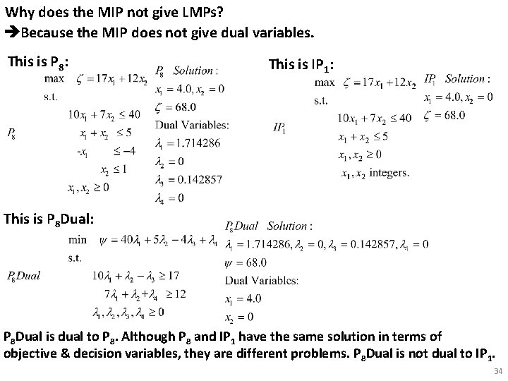
Why does the MIP not give LMPs? Because the MIP does not give dual variables. This is P 8: This is IP 1: This is P 8 Dual: P 8 Dual is dual to P 8. Although P 8 and IP 1 have the same solution in terms of objective & decision variables, they are different problems. P 8 Dual is not dual to IP 1. 34

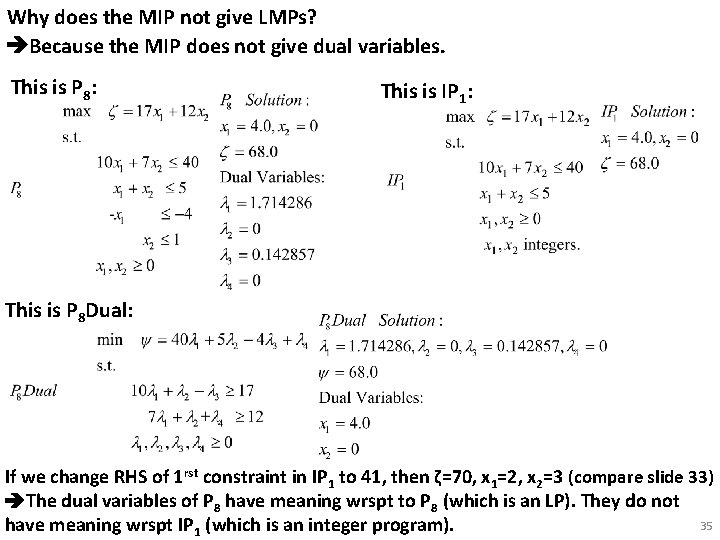
Why does the MIP not give LMPs? Because the MIP does not give dual variables. This is P 8: This is IP 1: This is P 8 Dual: If we change RHS of 1 rst constraint in IP 1 to 41, then ζ=70, x 1=2, x 2=3 (compare slide 33) The dual variables of P 8 have meaning wrspt to P 8 (which is an LP). They do not 35 have meaning wrspt IP 1 (which is an integer program).

Last Comment: There is a very good, but concise, description/ explanation of the MIP branch and bound method here: www. gurobi. com/resource/mip-basics/ (I also have it in a file on my computer 2019 class notes). It differs from my previous notes in this slide deck mainly in that it refers to a minimization problem, whereas I referred to a maximization problem. It is often helpful to see two different treatments of the same material. Read through the material in the above link and compare/contrast to the presentation of these slides; if it all makes sense to you, then you can feel confident. 36