Managerial Decision Making Chapter 6 Integer Linear Programming

Managerial Decision Making Chapter 6 Integer Linear Programming

Introduction When one or more variables in an LP problem must assume an integer value we have an Integer Linear Programming (ILP) problem. ILPs occur frequently: Number of workers, planes, machines, etc. must be integer. 0 -1 selection of projects, workers, advertisements. Fixed cost must be paid, fixed resource quantity must be used. Integer variables also allow us to build more accurate models for a number of common business problems.

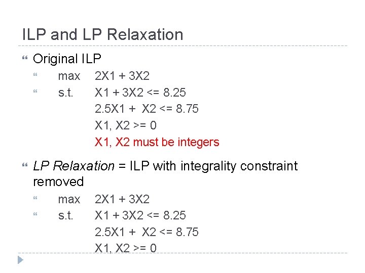
ILP and LP Relaxation Original ILP max s. t. 2 X 1 + 3 X 2 <= 8. 25 2. 5 X 1 + X 2 <= 8. 75 X 1, X 2 >= 0 X 1, X 2 must be integers LP Relaxation = ILP with integrality constraint removed max s. t. 2 X 1 + 3 X 2 <= 8. 25 2. 5 X 1 + X 2 <= 8. 75 X 1, X 2 >= 0

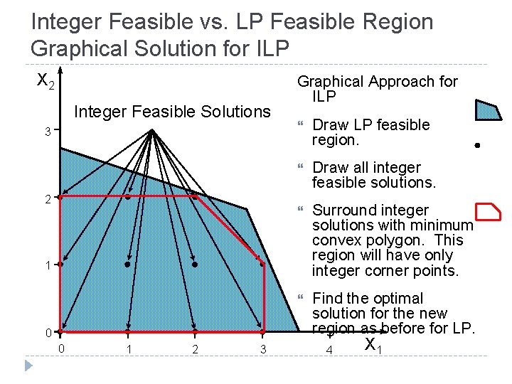
Integer Feasible vs. LP Feasible Region Graphical Solution for ILP X 2 Integer Feasible Solutions 3 2 Graphical Approach for ILP Draw LP feasible region. Draw all integer feasible solutions. Surround integer solutions with minimum convex polygon. This region will have only integer corner points. Find the optimal solution for the new region as before for LP. 1 0 0 1 2 3 4 X 1

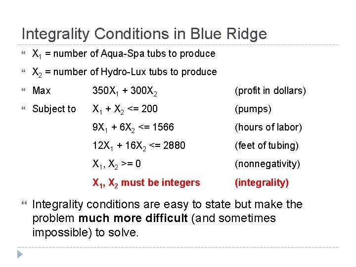
Integrality Conditions in Blue Ridge X 1 = number of Aqua-Spa tubs to produce X 2 = number of Hydro-Lux tubs to produce Max 350 X 1 + 300 X 2 (profit in dollars) Subject to X 1 + X 2 <= 200 (pumps) 9 X 1 + 6 X 2 <= 1566 (hours of labor) 12 X 1 + 16 X 2 <= 2880 (feet of tubing) X 1, X 2 >= 0 (nonnegativity) X 1, X 2 must be integers (integrality) Integrality conditions are easy to state but make the problem much more difficult (and sometimes impossible) to solve.

Solving ILP Problems In Network LP problems solutions are always integer, but in other LP problems solutions may be fractional. When solving an LP relaxation, sometimes you “get lucky” and obtain an integer feasible solution. This was the case in the original Blue Ridge Hot Tubs problem in earlier chapters. But what if we reduce the amount of labor available to 1520 hours and the amount of tubing to 2650 feet? See file Fig 6 -2. xls

Bounds The optimal solution to an LP relaxation gives a bound on the optimal objective function value of the ILP problem. The optimal solution of an ILP problem will not be better than the optimal solution of the LP relaxation. For maximization problems, the optimal relaxed objective function value is an upper bound on the optimal integer value. For minimization problems, the optimal relaxed objective function value is a lower bound on the optimal integer value.

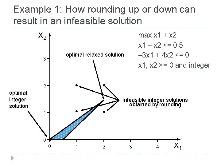
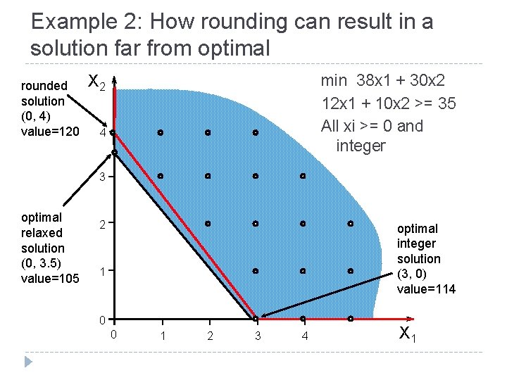
Rounding It is tempting to simply round a fractional solution to the closest integer solution. In general, this does not work reliably: The rounded solution may be infeasible. The rounded solution may be suboptimal.

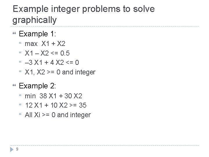
Example integer problems to solve graphically Example 1: max X 1 + X 2 X 1 – X 2 <= 0. 5 – 3 X 1 + 4 X 2 <= 0 X 1, X 2 >= 0 and integer Example 2: 9 min 38 X 1 + 30 X 2 12 X 1 + 10 X 2 >= 35 All Xi >= 0 and integer

Example 1: How rounding up or down can result in an infeasible solution X 2 max x 1 + x 2 x 1 – x 2 <= 0. 5 – 3 x 1 + 4 x 2 <= 0 x 1, x 2 >= 0 and integer optimal relaxed solution 3 2 optimal integer solution Infeasible integer solutions obtained by rounding 1 0 0 1 2 3 4 X 1

Example 2: How rounding can result in a solution far from optimal rounded solution (0, 4) value=120 X 2 min 38 x 1 + 30 x 2 12 x 1 + 10 x 2 >= 35 All xi >= 0 and integer 4 3 optimal relaxed solution (0, 3. 5) value=105 2 optimal integer solution (3, 0) value=114 1 0 0 1 2 3 4 X 1

Branch-and-Bound Algorithm for ILP The Branch-and-Bound (B&B) algorithm is the most common algorithm for solving ILP problems. B&B requires the solution of a series of LP problems termed “candidate problems”. Theoretically, B&B can solve any ILP. Practically, it often takes lots of computational effort (and time).

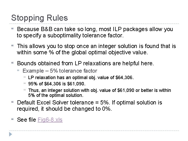
Stopping Rules Because B&B can take so long, most ILP packages allow you to specify a suboptimality tolerance factor. This allows you to stop once an integer solution is found that is within some % of the global optimal objective value. Bounds obtained from LP relaxations are helpful here. Example – 5% tolerance factor LP relaxation has an optimal obj. value of $64, 306. 95% of $64, 306 is $61, 090. Thus, an integer solution with obj. value of $61, 090 or better is within 5% of the optimal solution. Default Excel Solver tolerance = 5%. If optimal solution is required, it should be changed to 0%. See file Fig 6 -8. xls

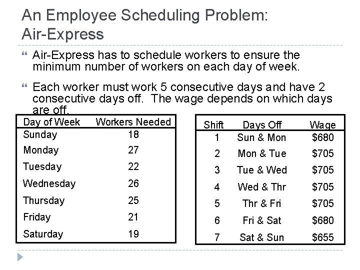
An Employee Scheduling Problem: Air-Express has to schedule workers to ensure the minimum number of workers on each day of week. Each worker must work 5 consecutive days and have 2 consecutive days off. The wage depends on which days are off. Day of Week Sunday Workers Needed 18 Shift 1 Days Off Sun & Mon Wage $680 Monday 27 2 Mon & Tue $705 Tuesday 22 3 Tue & Wed $705 Wednesday 26 4 Wed & Thr $705 Thursday 25 5 Thr & Fri $705 Friday 21 6 Fri & Sat $680 Saturday 19 7 Sat & Sun $655

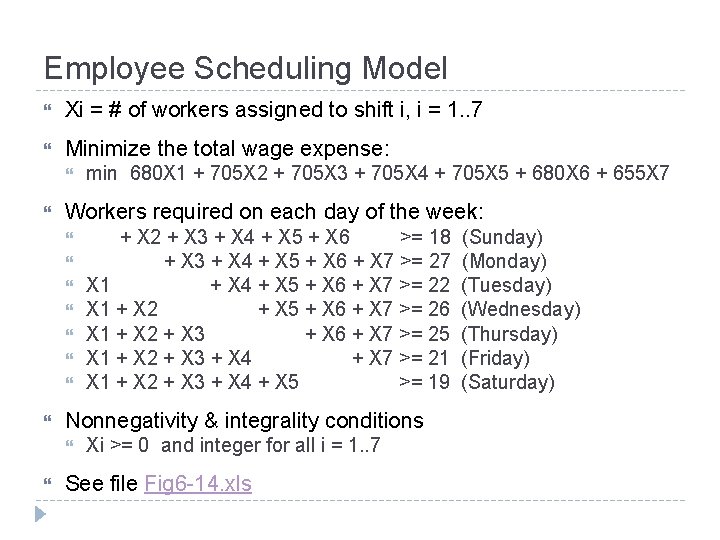
Employee Scheduling Model Xi = # of workers assigned to shift i, i = 1. . 7 Minimize the total wage expense: Workers required on each day of the week: + X 2 + X 3 + X 4 + X 5 + X 6 >= 18 + X 3 + X 4 + X 5 + X 6 + X 7 >= 27 X 1 + X 4 + X 5 + X 6 + X 7 >= 22 X 1 + X 2 + X 5 + X 6 + X 7 >= 26 X 1 + X 2 + X 3 + X 6 + X 7 >= 25 X 1 + X 2 + X 3 + X 4 + X 7 >= 21 X 1 + X 2 + X 3 + X 4 + X 5 >= 19 Nonnegativity & integrality conditions min 680 X 1 + 705 X 2 + 705 X 3 + 705 X 4 + 705 X 5 + 680 X 6 + 655 X 7 Xi >= 0 and integer for all i = 1. . 7 See file Fig 6 -14. xls (Sunday) (Monday) (Tuesday) (Wednesday) (Thursday) (Friday) (Saturday)

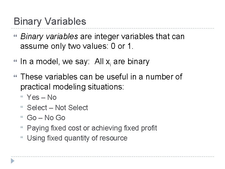
Binary Variables Binary variables are integer variables that can assume only two values: 0 or 1. In a model, we say: All xi are binary These variables can be useful in a number of practical modeling situations: Yes – No Select – Not Select Go – No Go Paying fixed cost or achieving fixed profit Using fixed quantity of resource

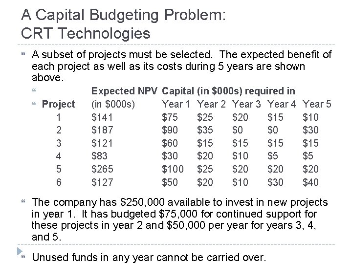
A Capital Budgeting Problem: CRT Technologies A subset of projects must be selected. The expected benefit of each project as well as its costs during 5 years are shown above. Project 1 2 3 4 5 6 Expected NPV (in $000 s) $141 $187 $121 $83 $265 $127 Capital (in $000 s) required in Year 1 Year 2 Year 3 Year 4 $75 $20 $15 $90 $35 $0 $0 $60 $15 $15 $30 $20 $10 $5 $100 $25 $20 $50 $20 $10 $30 Year 5 $10 $30 $15 $5 $20 $40 The company has $250, 000 available to invest in new projects in year 1. It has budgeted $75, 000 for continued support for these projects in year 2 and $50, 000 per year for years 3, 4, and 5. Unused funds in any year cannot be carried over.

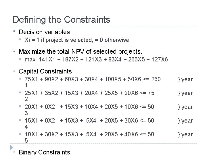
Defining the Constraints Decision variables Maximize the total NPV of selected projects. max 141 X 1 + 187 X 2 + 121 X 3 + 83 X 4 + 265 X 5 + 127 X 6 Capital Constraints Xi = 1 if project is selected; = 0 otherwise 75 X 1 + 90 X 2 + 60 X 3 + 30 X 4 + 100 X 5 + 50 X 6 <= 250 1 25 X 1 + 35 X 2 + 15 X 3 + 20 X 4 + 25 X 5 + 20 X 6 <= 75 2 20 X 1 + 0 X 2 + 15 X 3 + 10 X 4 + 20 X 5 + 10 X 6 <= 50 3 15 X 1 + 0 X 2 + 15 X 3 + 5 X 4 + 20 X 5 + 30 X 6 <= 50 4 10 X 1 + 30 X 2 + 15 X 3 + 5 X 4 + 20 X 5 + 40 X 6 <= 50 5 Binary Constraints } year } year

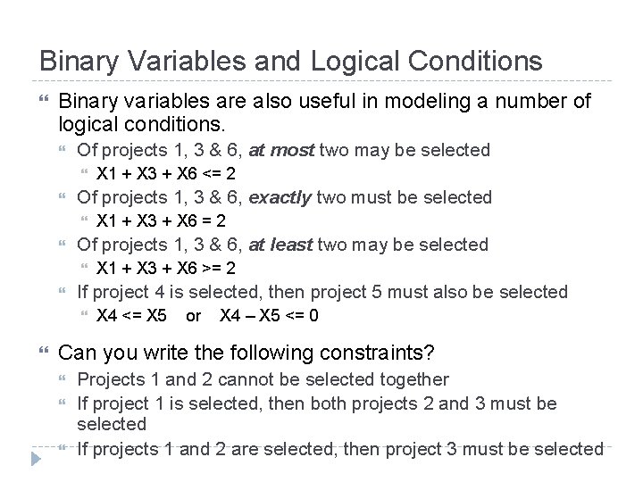
Binary Variables and Logical Conditions Binary variables are also useful in modeling a number of logical conditions. Of projects 1, 3 & 6, at most two may be selected Of projects 1, 3 & 6, exactly two must be selected X 1 + X 3 + X 6 >= 2 If project 4 is selected, then project 5 must also be selected X 1 + X 3 + X 6 = 2 Of projects 1, 3 & 6, at least two may be selected X 1 + X 3 + X 6 <= 2 X 4 <= X 5 or X 4 – X 5 <= 0 Can you write the following constraints? Projects 1 and 2 cannot be selected together If project 1 is selected, then both projects 2 and 3 must be selected If projects 1 and 2 are selected, then project 3 must be selected

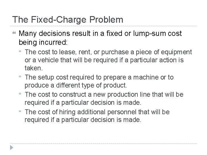
The Fixed-Charge Problem Many decisions result in a fixed or lump-sum cost being incurred: The cost to lease, rent, or purchase a piece of equipment or a vehicle that will be required if a particular action is taken. The setup cost required to prepare a machine or to produce a different type of product. The cost to construct a new production line that will be required if a particular decision is made. The cost of hiring additional personnel that will be required if a particular decision is made.

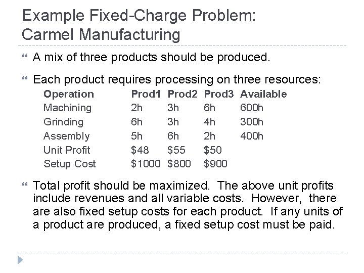
Example Fixed-Charge Problem: Carmel Manufacturing A mix of three products should be produced. Each product requires processing on three resources: Operation Machining Grinding Assembly Unit Profit Setup Cost Prod 1 2 h 6 h 5 h $48 $1000 Prod 2 3 h 3 h 6 h $55 $800 Prod 3 6 h 4 h 2 h $50 $900 Available 600 h 300 h 400 h Total profit should be maximized. The above unit profits include revenues and all variable costs. However, there also fixed setup costs for each product. If any units of a product are produced, a fixed setup cost must be paid.

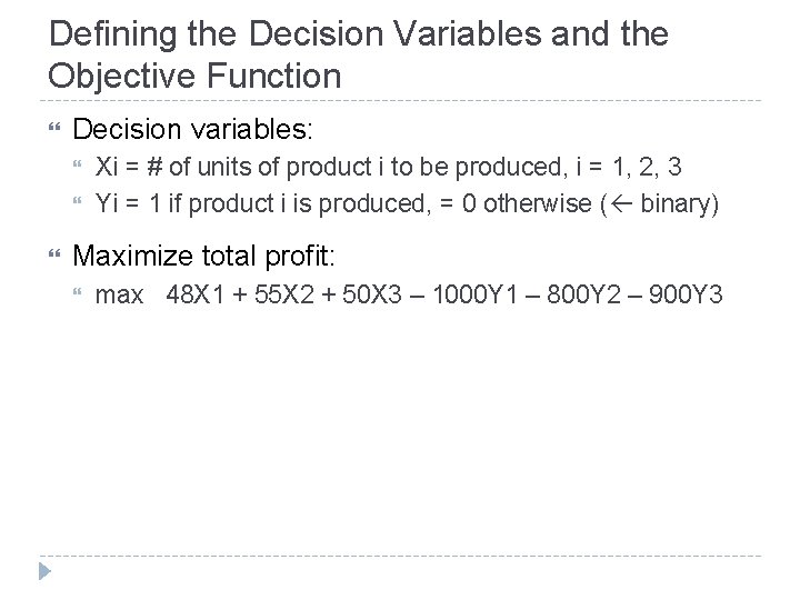
Defining the Decision Variables and the Objective Function Decision variables: Xi = # of units of product i to be produced, i = 1, 2, 3 Yi = 1 if product i is produced, = 0 otherwise ( binary) Maximize total profit: max 48 X 1 + 55 X 2 + 50 X 3 – 1000 Y 1 – 800 Y 2 – 900 Y 3

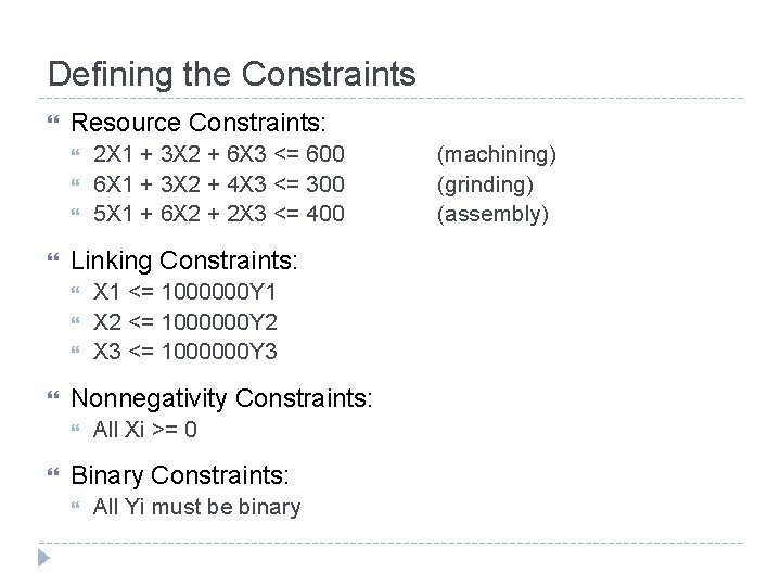
Defining the Constraints Resource Constraints: Linking Constraints: X 1 <= 1000000 Y 1 X 2 <= 1000000 Y 2 X 3 <= 1000000 Y 3 Nonnegativity Constraints: 2 X 1 + 3 X 2 + 6 X 3 <= 600 6 X 1 + 3 X 2 + 4 X 3 <= 300 5 X 1 + 6 X 2 + 2 X 3 <= 400 All Xi >= 0 Binary Constraints: All Yi must be binary (machining) (grinding) (assembly)

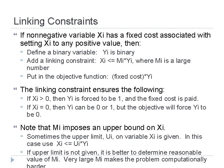
Linking Constraints If nonnegative variable Xi has a fixed cost associated with setting Xi to any positive value, then: The linking constraint ensures the following: Define a binary variable: Yi is binary Add a linking constraint: Xi <= Mi*Yi, where Mi is a large number Put in the objective function: (fixed cost)*Yi If Xi > 0, then Yi is forced to be 1, and the fixed cost is paid. If Xi = 0, then Yi can be 0 or 1, but the objective will force Yi to be 0. Note that Mi imposes an upper bound on Xi. Sometimes the upper limit, Ui, on variable Xi is given. In this case use Xi <= Ui*Yi If upper limit is not given, it is better to determine reasonable value of Mi. Very large Mi makes the problem computationally

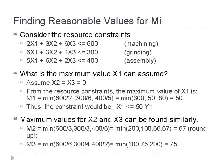
Finding Reasonable Values for Mi Consider the resource constraints (machining) (grinding) (assembly) What is the maximum value X 1 can assume? 2 X 1 + 3 X 2 + 6 X 3 <= 600 6 X 1 + 3 X 2 + 4 X 3 <= 300 5 X 1 + 6 X 2 + 2 X 3 <= 400 Assume X 2 = X 3 = 0 From the resource constraints, the maximum value of X 1 is: M 1 = min(600/2, 300/6, 400/5) = min(300, 50, 80) = 50. Thus, the constraint would be: X 1 <= 50 Y 1 Maximum values for X 2 and X 3 can be found similarly. M 2 = min(600/3, 300/3, 400/6)= min(200, 100, 66. 67) = 67 (round up!) M 3 = min(600/6, 300/4, 400/2)= min(100, 75, 200) = 75.

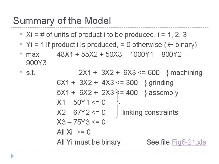
Summary of the Model Xi = # of units of product i to be produced, i = 1, 2, 3 Yi = 1 if product i is produced, = 0 otherwise ( binary) max 48 X 1 + 55 X 2 + 50 X 3 – 1000 Y 1 – 800 Y 2 – 900 Y 3 s. t. 2 X 1 + 3 X 2 + 6 X 3 <= 600 } machining 6 X 1 + 3 X 2 + 4 X 3 <= 300 } grinding 5 X 1 + 6 X 2 + 2 X 3 <= 400 } assembly X 1 – 50 Y 1 <= 0 X 2 – 67 Y 2 <= 0 linking constraints X 3 – 75 Y 3 <= 0 All Xi >= 0 All Yi must be binary See file Fig 6 -21. xls

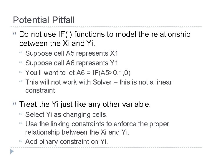
Potential Pitfall Do not use IF( ) functions to model the relationship between the Xi and Yi. Suppose cell A 5 represents X 1 Suppose cell A 6 represents Y 1 You’ll want to let A 6 = IF(A 5>0, 1, 0) This will not work with Solver – this is not a linear constraint! Treat the Yi just like any other variable. Select Yi as changing cells. Use the linking constraints to enforce the proper relationship between the Xi and Yi. Add binary constraint on Yi.

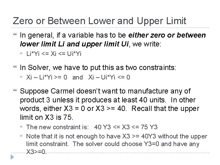
Zero or Between Lower and Upper Limit In general, if a variable has to be either zero or between lower limit Li and upper limit Ui, we write: In Solver, we have to put this as two constraints: Li*Yi <= Xi <= Ui*Yi Xi – Li*Yi >= 0 and Xi – Ui*Yi <= 0 Suppose Carmel doesn’t want to manufacture any of product 3 unless it produces at least 40 units. In other words, either X 3 = 0 or X 3 >= 40. Recall that the upper limit on X 3 is 75. The new constraint is: 40 Y 3 <= X 3 <= 75 Y 3 Note that it is not enough to have X 3 >= 40 Y 3 without the upper limit constraint. The solver could choose Y 3=0 and have any X 3>=0.

Chapter 6 Summary Integrality constraints make linear problems much harder to solve. Rounding fractional solution to integer values is not guaranteed to give optimal or even feasible solution. Binary variables are useful for a number of yes-no decision problems. Logical conditions can be expressed. Binary variables with linking constraints can be used if: Fixed costs should be paid. Variables should be zero or between lower and upper limits.