EEEcon 458 Introduction to Linear Programming J Mc

EE/Econ 458 Introduction to Linear Programming J. Mc. Calley 1

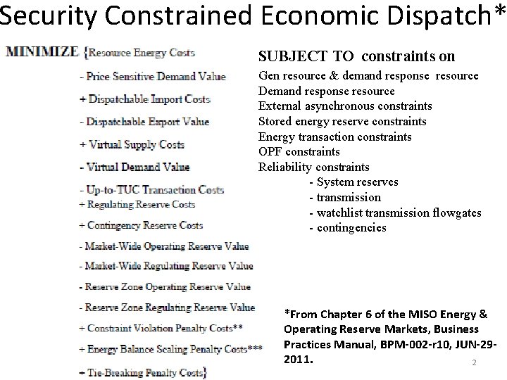
Security Constrained Economic Dispatch* SUBJECT TO constraints on Gen resource & demand response resource Demand response resource External asynchronous constraints Stored energy reserve constraints Energy transaction constraints OPF constraints Reliability constraints - System reserves - transmission - watchlist transmission flowgates - contingencies *From Chapter 6 of the MISO Energy & Operating Reserve Markets, Business Practices Manual, BPM-002 -r 10, JUN-292011. 2

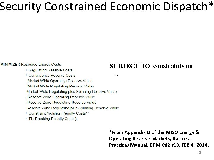
Security Constrained Economic Dispatch* SUBJECT TO constraints on … *From Appendix D of the MISO Energy & Operating Reserve Markets, Business Practices Manual, BPM-002 -r 13, FEB 4, -2014. 3

Security Constrained Economic Dispatch* SUBJECT TO constraints on … *From Attachment D of the MISO Energy & Operating Reserve Markets, Business Practices Manual, BPM-002 -r 18, Sept 23, -2017. See https: //www. misoenergy. org/legal/business-practice-manuals/8 4

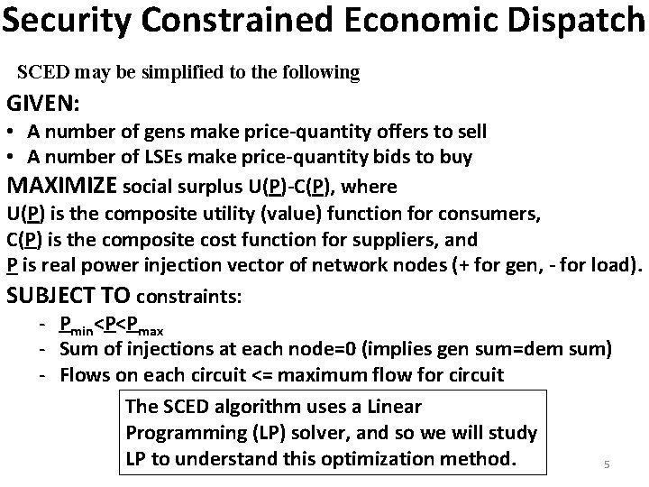
Security Constrained Economic Dispatch SCED may be simplified to the following GIVEN: • A number of gens make price-quantity offers to sell • A number of LSEs make price-quantity bids to buy MAXIMIZE social surplus U(P)-C(P), where U(P) is the composite utility (value) function for consumers, C(P) is the composite cost function for suppliers, and P is real power injection vector of network nodes (+ for gen, - for load). SUBJECT TO constraints: - Pmin<P<Pmax - Sum of injections at each node=0 (implies gen sum=dem sum) - Flows on each circuit <= maximum flow for circuit The SCED algorithm uses a Linear Programming (LP) solver, and so we will study LP to understand this optimization method. 5

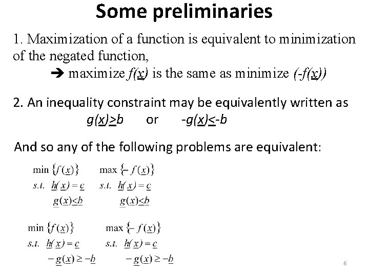
Some preliminaries 1. Maximization of a function is equivalent to minimization of the negated function, maximize f(x) is the same as minimize (-f(x)) 2. An inequality constraint may be equivalently written as g(x)>b or -g(x)<-b And so any of the following problems are equivalent: 6

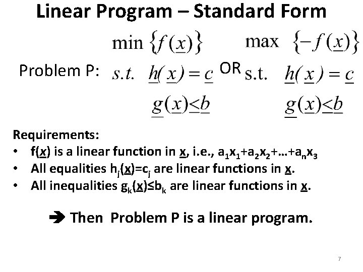
Linear Program – Standard Form Problem P: OR Requirements: • f(x) is a linear function in x, i. e. , a 1 x 1+a 2 x 2+…+anx 3 • All equalities hj(x)=cj are linear functions in x. • All inequalities gk(x)≤bk are linear functions in x. Then Problem P is a linear program. 7

Linear Program – A Convex Program Problem P: Feasible set Recall: If f(x) is a convex function, and if S is a convex set, then the above problem is a convex programming problem. f(x) is linear, therefore a convex function. If S is formed by inequalities, it is polyhedral (many flat faces), therefore convex. One linear equality reduces feasible set S to the line. More than one reduces feasible set S to their intersections. S is convex in both cases. A linear program is a convex programming problem. If we find a locally optimal solution, it will be globally optimal. 8

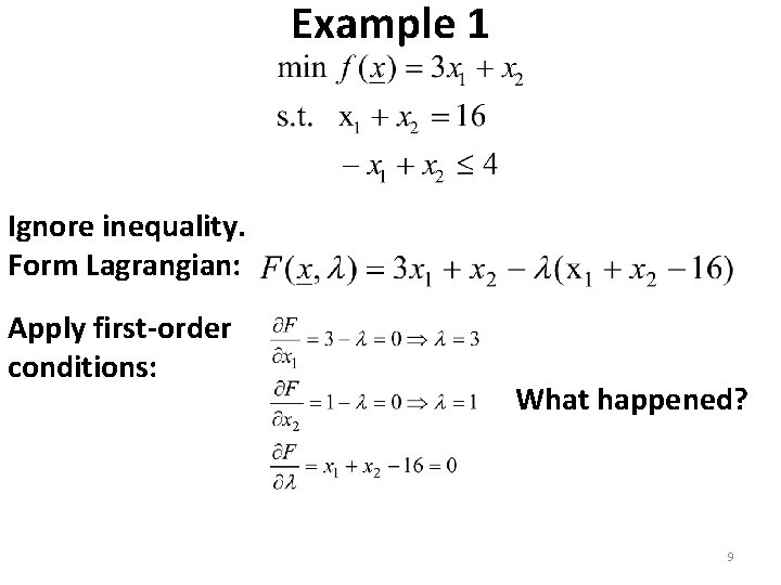
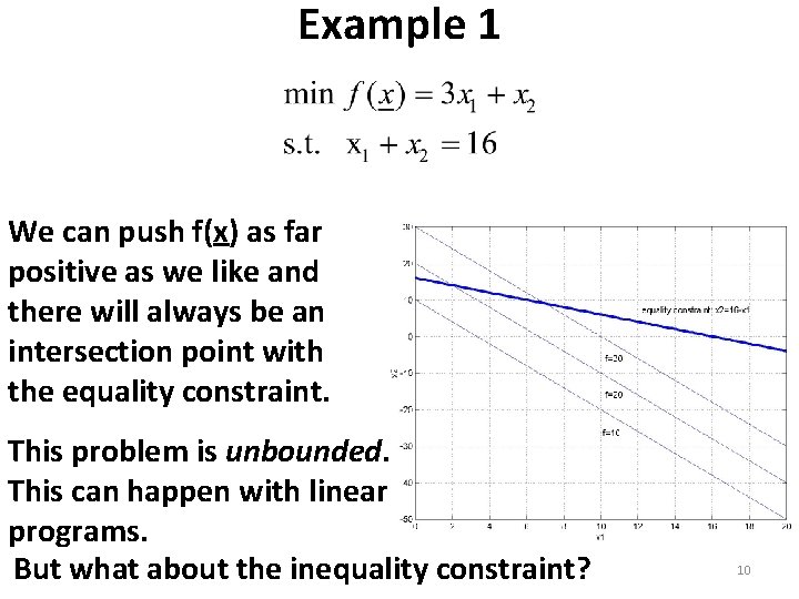
Example 1 Ignore inequality. Form Lagrangian: Apply first-order conditions: What happened? 9

Example 1 We can push f(x) as far positive as we like and there will always be an intersection point with the equality constraint. This problem is unbounded. This can happen with linear programs. But what about the inequality constraint? 10

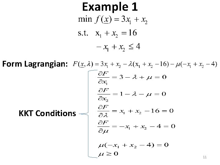
Example 1 Form Lagrangian: KKT Conditions 11

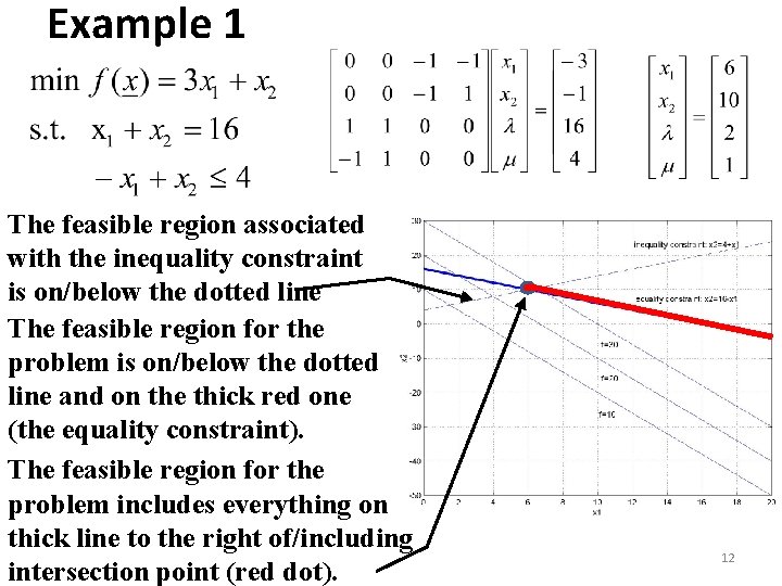
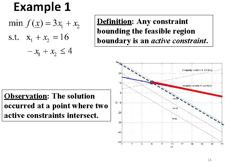
Example 1 The feasible region associated with the inequality constraint is on/below the dotted line The feasible region for the problem is on/below the dotted line and on the thick red one (the equality constraint). The feasible region for the problem includes everything on thick line to the right of/including intersection point (red dot). 12

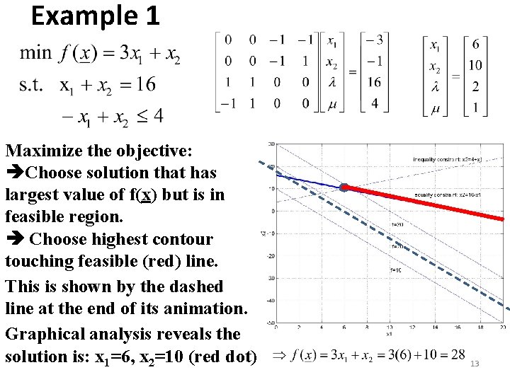
Example 1 Maximize the objective: Choose solution that has largest value of f(x) but is in feasible region. Choose highest contour touching feasible (red) line. This is shown by the dashed line at the end of its animation. Graphical analysis reveals the solution is: x 1=6, x 2=10 (red dot) 13

Example 1 Definition: Any constraint bounding the feasible region boundary is an active constraint. Observation: The solution occurred at a point where two active constraints intersect. 14

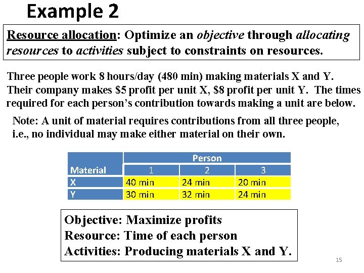
Example 2 Resource allocation: Optimize an objective through allocating resources to activities subject to constraints on resources. Three people work 8 hours/day (480 min) making materials X and Y. Their company makes $5 profit per unit X, $8 profit per unit Y. The times required for each person’s contribution towards making a unit are below. Note: A unit of material requires contributions from all three people, i. e. , no individual may make either material on their own. Material X Y 1 40 min 30 min Person 2 24 min 32 min 3 20 min 24 min Objective: Maximize profits Resource: Time of each person Activities: Producing materials X and Y. 15

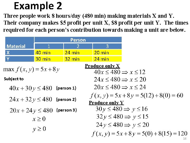
Example 2 Three people work 8 hours/day (480 min) making materials X and Y. Their company makes $5 profit per unit X, $8 profit per unit Y. The times required for each person’s contribution towards making a unit are below. Material X Y 1 40 min 30 min Person 2 3 24 min 20 min 32 min 24 min Produce only X Subject to (person 1) (person 2) Produce only Y (person 3) 16

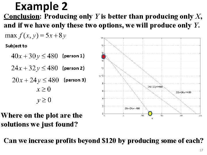
Example 2 Conclusion: Producing only Y is better than producing only X, and if we have only these two options, we will produce only Y. Subject to (person 1) (person 2) (person 3) Where on the plot are the solutions we just found? Can we increase profits beyond $120 by producing some of each? 17

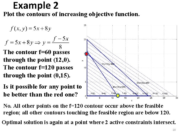
Example 2 Plot the contours of increasing objective function. The contour f=60 passes through the point (12, 0). The contour f=120 passes through the point (0, 15). Is it possible for any point to be better than the red one? No. All other points on the f=120 contour occur above the feasible region; all other contours touching the feasible region are below 120. Optimal solution is again at a point where 2 active constraints intersect. 18

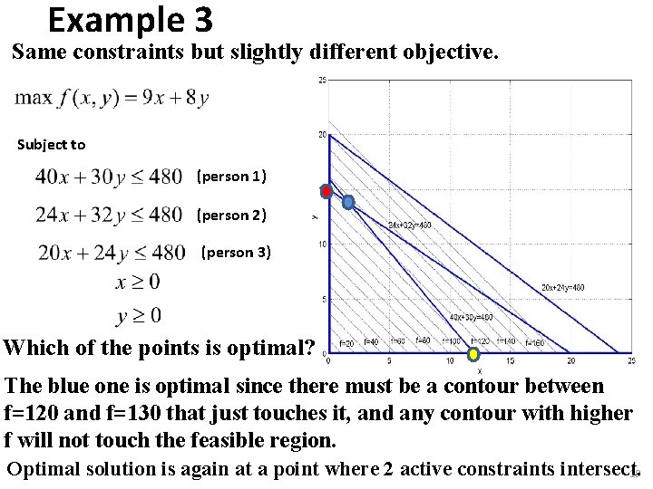
Example 3 Same constraints but slightly different objective. Subject to (person 1) (person 2) (person 3) Which of the points is optimal? The blue one is optimal since there must be a contour between f=120 and f=130 that just touches it, and any contour with higher f will not touch the feasible region. Optimal solution is again at a point where 2 active constraints intersect. 19

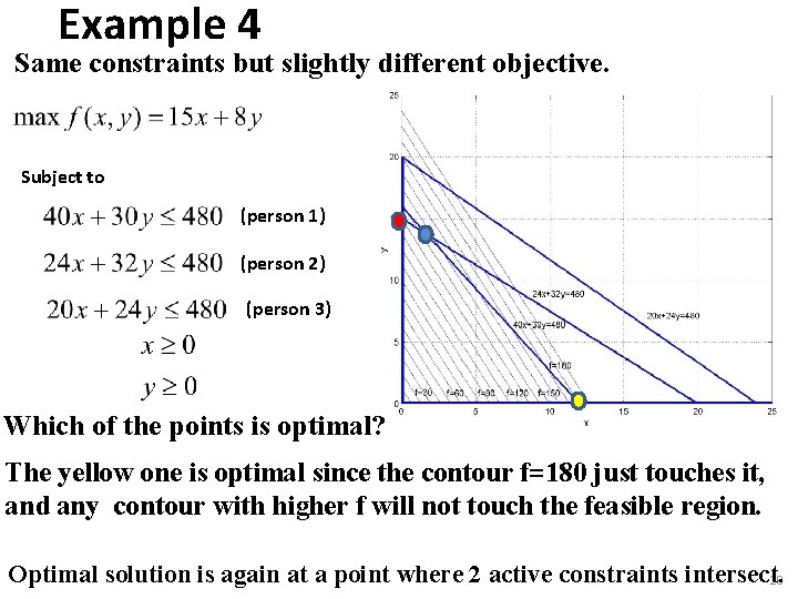
Example 4 Same constraints but slightly different objective. Subject to (person 1) (person 2) (person 3) Which of the points is optimal? The yellow one is optimal since the contour f=180 just touches it, and any contour with higher f will not touch the feasible region. Optimal solution is again at a point where 2 active constraints intersect. 20

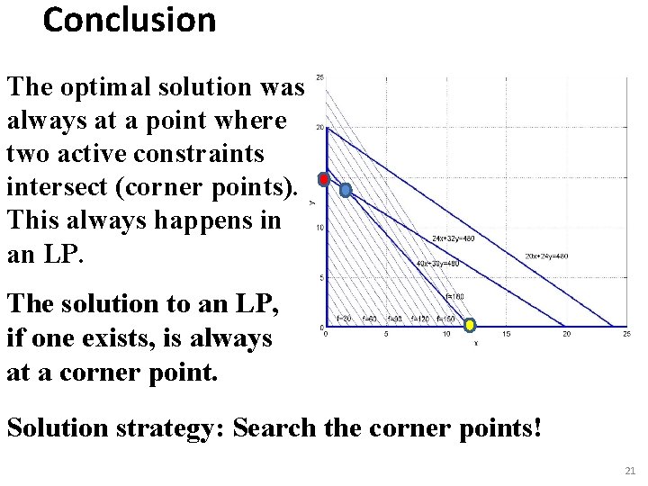
Conclusion The optimal solution was always at a point where two active constraints intersect (corner points). This always happens in an LP. The solution to an LP, if one exists, is always at a corner point. Solution strategy: Search the corner points! 21

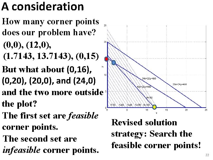
A consideration How many corner points does our problem have? (0, 0), (12, 0), (1. 7143, 13. 7143), (0, 15) But what about (0, 16), (0, 20), (20, 0), and (24, 0) and the two more outside the plot? The first set are feasible Revised solution corner points. strategy: Search the The second set are feasible corner points! infeasible corner points. 22

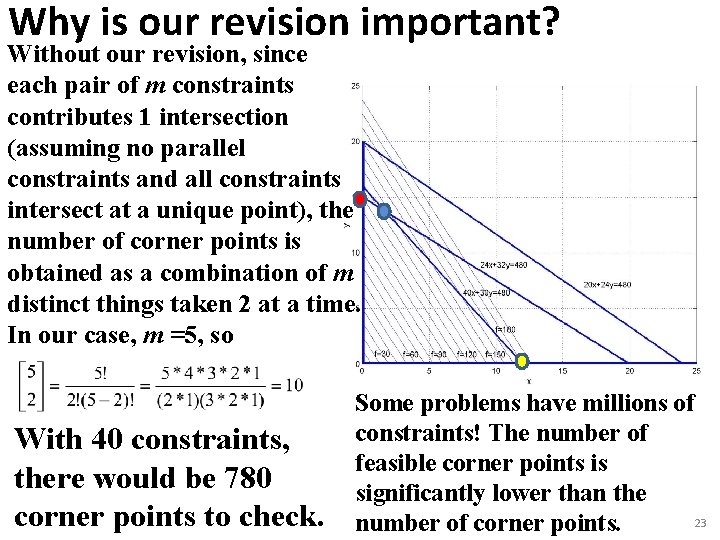
Why is our revision important? Without our revision, since each pair of m constraints contributes 1 intersection (assuming no parallel constraints and all constraints intersect at a unique point), the number of corner points is obtained as a combination of m distinct things taken 2 at a time. In our case, m =5, so With 40 constraints, there would be 780 corner points to check. Some problems have millions of constraints! The number of feasible corner points is significantly lower than the 23 number of corner points.

An approach Revised solution strategy: Search the feasible corner points! 24

An approach 1. Pick a feasible corner point at random. 2. Move to an adjacent feasible corner point that is better. a. If there are two that are better, move to the one that is best. b. If there are no better adjacent feasible corner points, the current feasible corner point is the solution to the problem. Optimality (stopping) condition: If a feasible corner point is equal to or better than all its adjacent feasible corner points, then it is equal to or better than all other feasible corner points, i. e. , it is optimal. Main ideas of proof: 1. If objective function monotonically increases (decreases) in some direction within the decision-vector space, then each adjacent corner point will become progressively better in the direction of objective function increase (decrease) such that the last corner point must have two adjacent corner points that are worse. 2. The monotonicity of objective function increase (decrease) is guaranteed by its linearity. 25

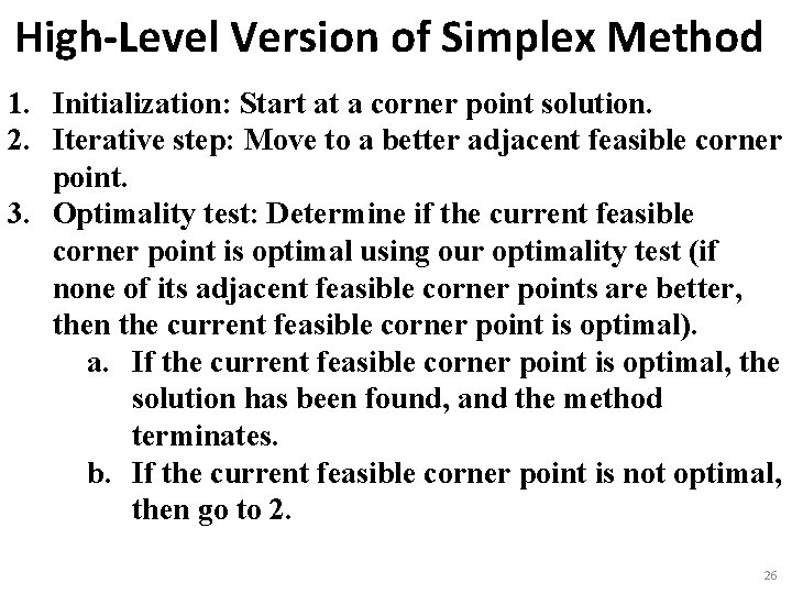
High-Level Version of Simplex Method 1. Initialization: Start at a corner point solution. 2. Iterative step: Move to a better adjacent feasible corner point. 3. Optimality test: Determine if the current feasible corner point is optimal using our optimality test (if none of its adjacent feasible corner points are better, then the current feasible corner point is optimal). a. If the current feasible corner point is optimal, the solution has been found, and the method terminates. b. If the current feasible corner point is not optimal, then go to 2. 26