EECS 274 Computer Vision Motion Estimation Motion estimation

EECS 274 Computer Vision Motion Estimation

Motion estimation • Aligning images • Estimate motion parameters • Optical flow – Lucas-Kanade algorithm – Horn-Schunck algorithm • Slides based on Szeliski’s lecture notes • Reading: FP Chapter 15, S Chapter 8

Why estimate visual motion? • Visual Motion can be annoying – Camera instabilities, jitter – Measure it; remove it (stabilize) • Visual Motion indicates dynamics in the scene – Moving objects, behavior – Track objects and analyze trajectories • Visual Motion reveals spatial layout – Motion parallax

Classes of techniques • Feature-based methods – Extract visual features (corners, textured areas) and track them – Sparse motion fields, but possibly robust tracking – Suitable especially when image motion is large (10 s of pixels) • Direct methods – Directly recover image motion from spatio-temporal image brightness variations – Global motion parameters directly recovered without an intermediate feature motion calculation – Dense motion fields, but more sensitive to appearance variations – Suitable for video and when image motion is small (< 10 pixels)

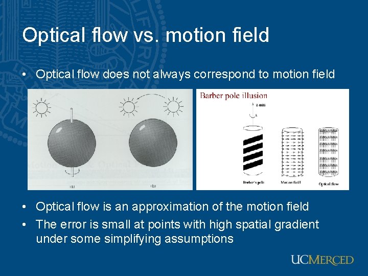
Optical flow vs. motion field • Optical flow does not always correspond to motion field • Optical flow is an approximation of the motion field • The error is small at points with high spatial gradient under some simplifying assumptions

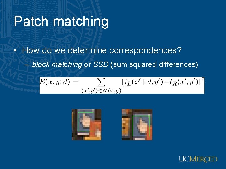
Patch matching • How do we determine correspondences? – block matching or SSD (sum squared differences)

Correlation and SSD • For larger displacements, do template matching – Define a small area around a pixel as the template – Match the template against each pixel within a search area in next image – Use a match measure such as correlation, normalized correlation, or sum-of-squares difference – Choose the maximum (or minimum) as the match – Sub-pixel estimate (Lucas-Kanade)

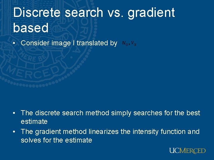
Discrete search vs. gradient based • Consider image I translated by • The discrete search method simply searches for the best estimate • The gradient method linearizes the intensity function and solves for the estimate

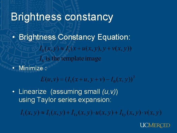
Brightness constancy • Brightness Constancy Equation: • Minimize : • Linearize (assuming small (u, v)) using Taylor series expansion:

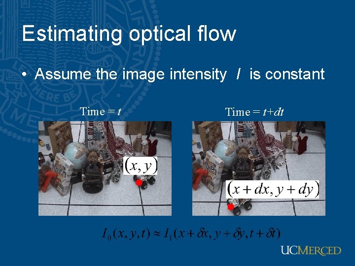
Estimating optical flow • Assume the image intensity I is constant Time = t+dt

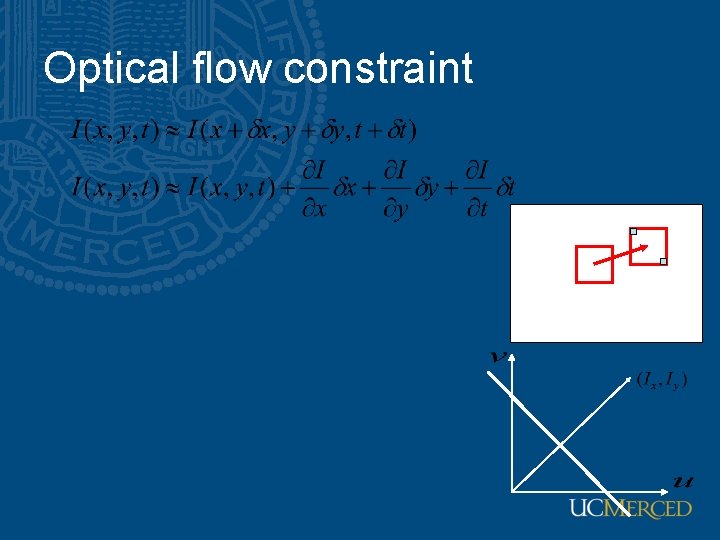
Optical flow constraint

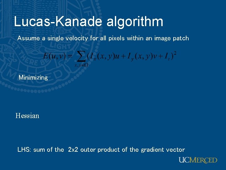
Lucas-Kanade algorithm Assume a single velocity for all pixels within an image patch Minimizing Hessian LHS: sum of the 2 x 2 outer product of the gradient vector

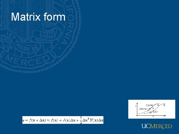
Matrix form

Matrix form for computational efficiency

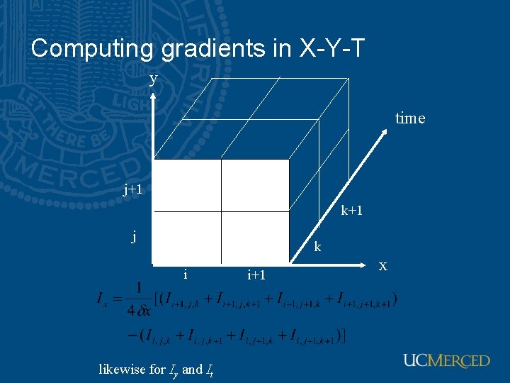
Computing gradients in X-Y-T y time j+1 k+1 j k i likewise for Iy and It i+1 x

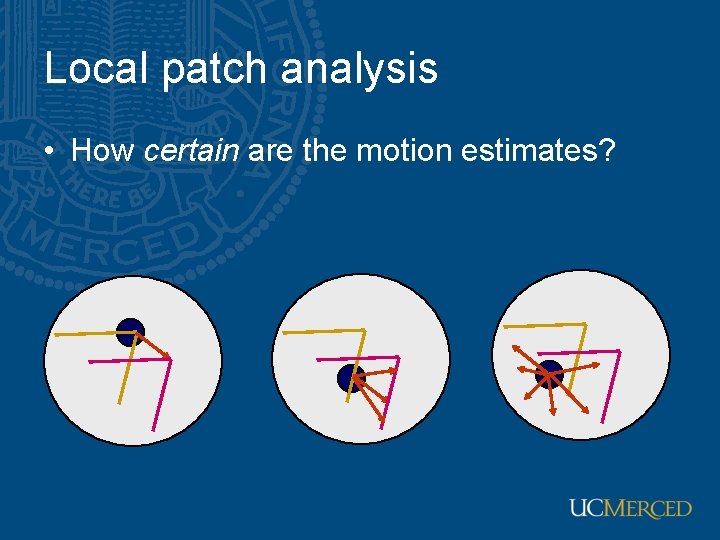
Local patch analysis • How certain are the motion estimates?

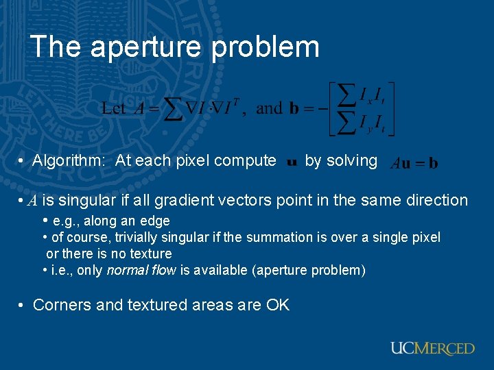
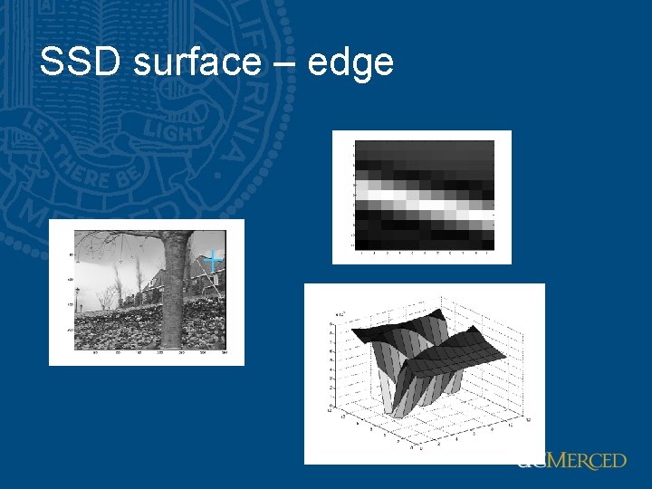
The aperture problem • Algorithm: At each pixel compute by solving • A is singular if all gradient vectors point in the same direction • e. g. , along an edge • of course, trivially singular if the summation is over a single pixel or there is no texture • i. e. , only normal flow is available (aperture problem) • Corners and textured areas are OK

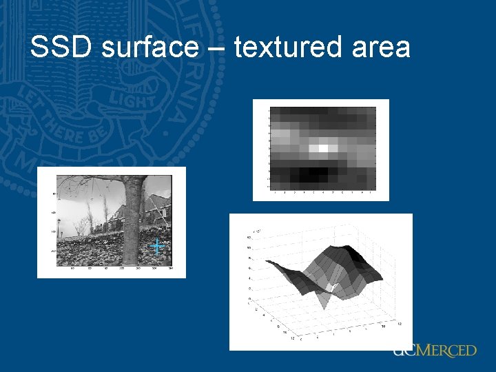
SSD surface – textured area

SSD surface – edge

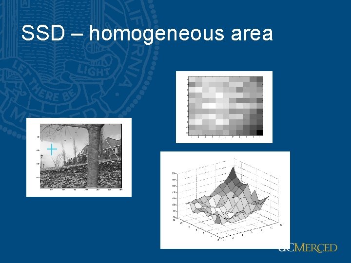
SSD – homogeneous area

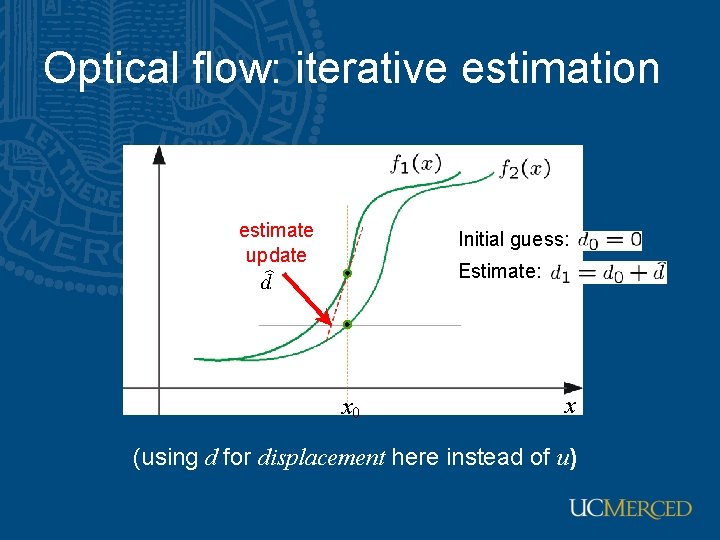
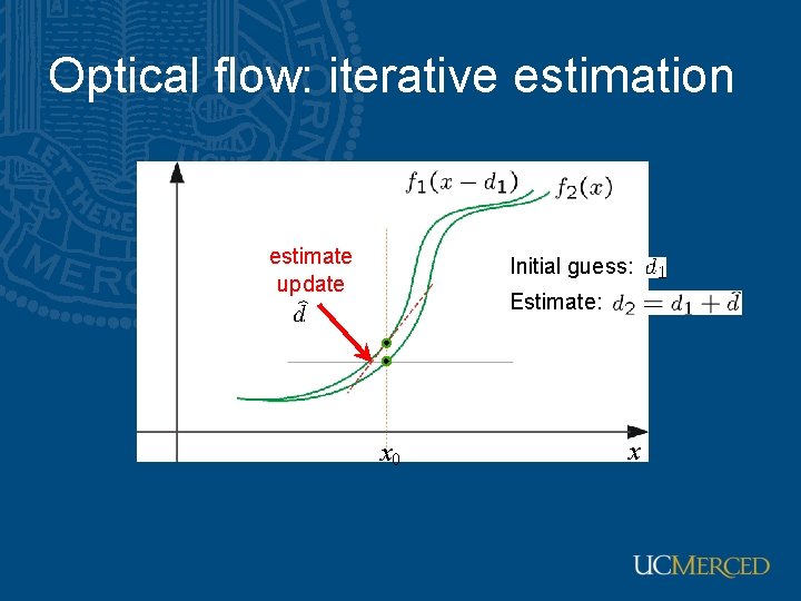
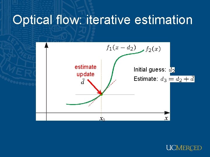
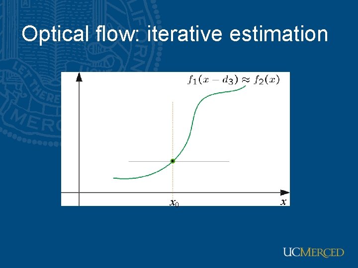
Iterative refinement • Estimate velocity at each pixel using one iteration of Lucas and Kanade estimation • Warp one image toward the other using the estimated flow field (easier said than done) • Refine estimate by repeating the process

Optical flow: iterative estimation estimate update Initial guess: Estimate: x 0 x (using d for displacement here instead of u)

Optical flow: iterative estimation estimate update Initial guess: Estimate: x 0 x

Optical flow: iterative estimation estimate update Initial guess: Estimate: x 0 x

Optical flow: iterative estimation x 0 x

Optical flow: iterative estimation • Some implementation issues: – Warping is not easy (ensure that errors in warping are smaller than the estimate refinement) – Warp one image, take derivatives of the other so you don’t need to re-compute the gradient after each iteration – Often useful to low-pass filter the images before motion estimation (for better derivative estimation, and linear approximations to image intensity)

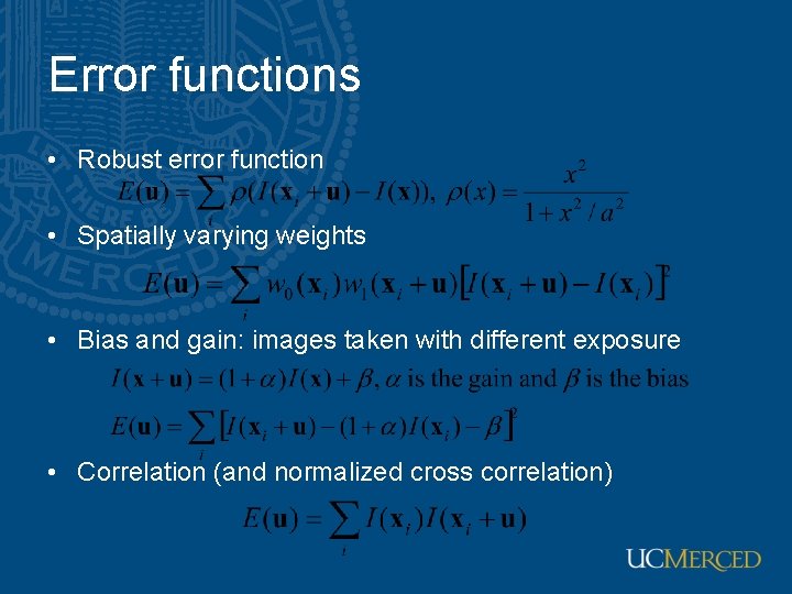
Error functions • Robust error function • Spatially varying weights • Bias and gain: images taken with different exposure • Correlation (and normalized cross correlation)

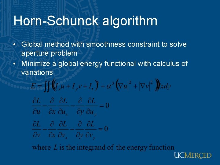
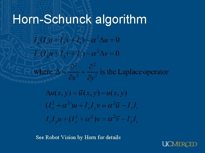
Horn-Schunck algorithm • Global method with smoothness constraint to solve aperture problem • Minimize a global energy functional with calculus of variations

Horn-Schunck algorithm See Robot Vision by Horn for details

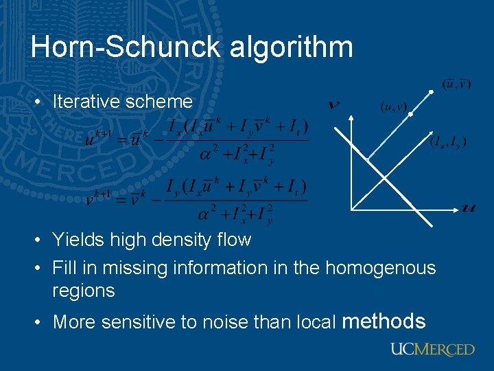
Horn-Schunck algorithm • Iterative scheme • Yields high density flow • Fill in missing information in the homogenous regions • More sensitive to noise than local methods

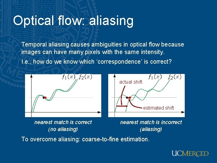
Optical flow: aliasing Temporal aliasing causes ambiguities in optical flow because images can have many pixels with the same intensity. I. e. , how do we know which ‘correspondence’ is correct? actual shift estimated shift nearest match is correct (no aliasing) nearest match is incorrect (aliasing) To overcome aliasing: coarse-to-fine estimation

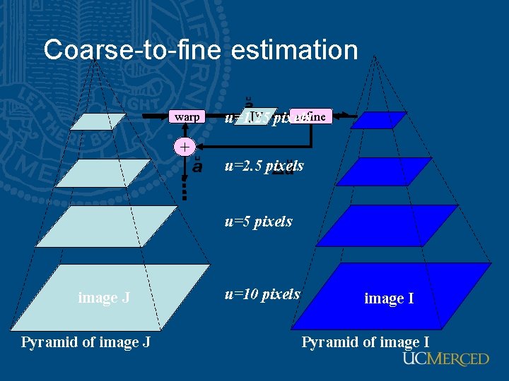
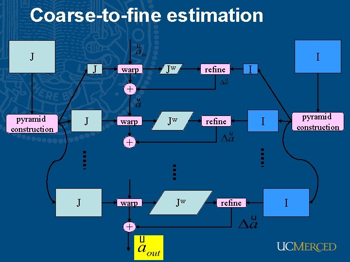
Coarse-to-fine estimation warp refine Jw pixels u=1. 25 + u=2. 5 pixels u=5 pixels image J Pyramid of image J u=10 pixels image I Pyramid of image I

Coarse-to-fine estimation J J warp Jw refine I I + pyramid construction J warp pyramid construction I + J warp + Jw refine I

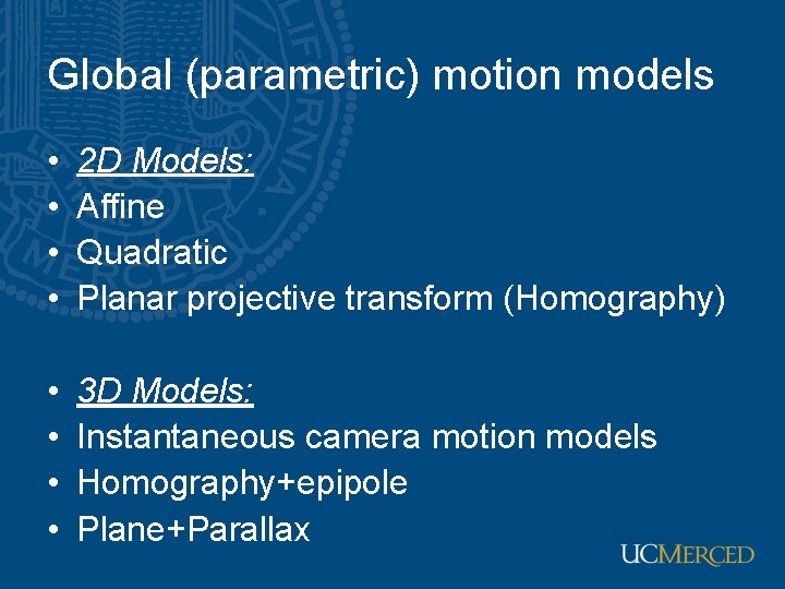
Global (parametric) motion models • • 2 D Models: Affine Quadratic Planar projective transform (Homography) • • 3 D Models: Instantaneous camera motion models Homography+epipole Plane+Parallax

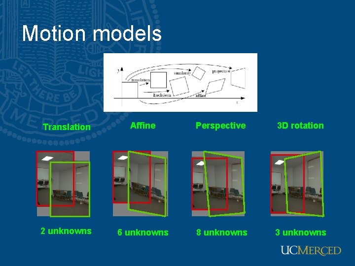
Motion models Translation Affine Perspective 3 D rotation 2 unknowns 6 unknowns 8 unknowns 3 unknowns

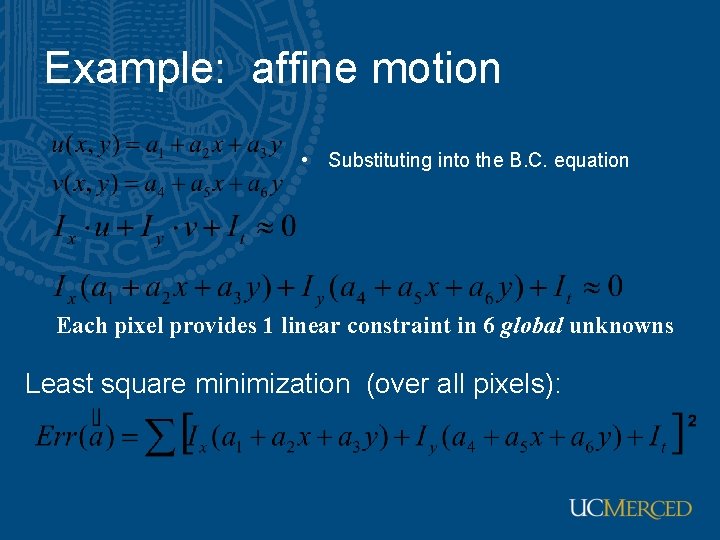
Example: affine motion • Substituting into the B. C. equation Each pixel provides 1 linear constraint in 6 global unknowns Least square minimization (over all pixels):

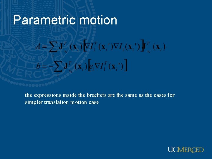
Parametric motion i. e. , the product of image gradient with Jacobian of the correspondence field

Parametric motion the expressions inside the brackets are the same as the cases for simpler translation motion case

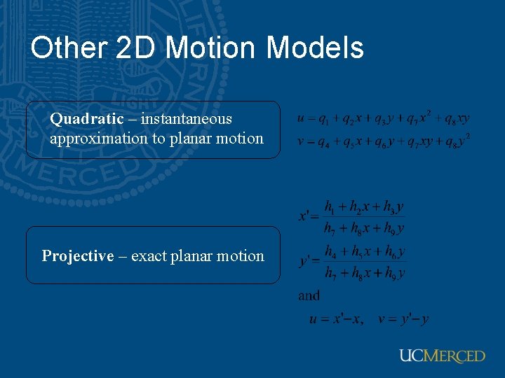
Other 2 D Motion Models Quadratic – instantaneous approximation to planar motion Projective – exact planar motion

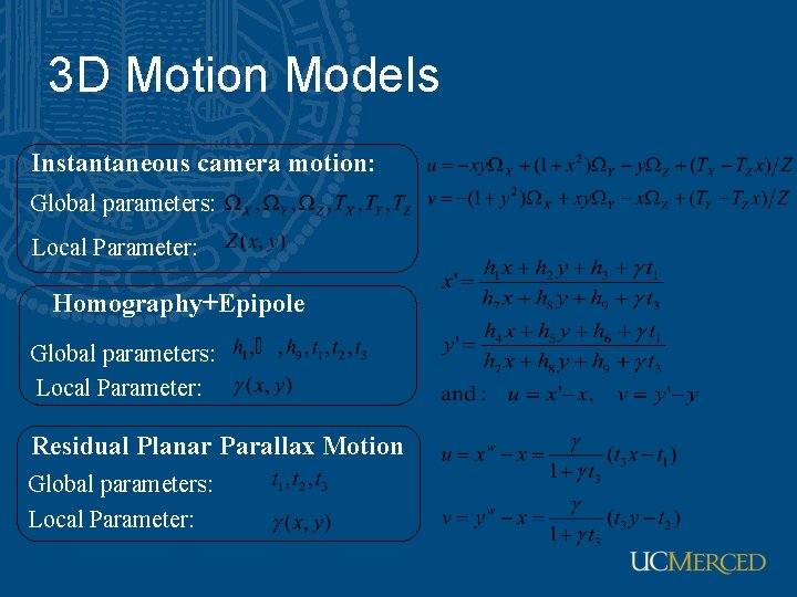
3 D Motion Models Instantaneous camera motion: Global parameters: Local Parameter: Homography+Epipole Global parameters: Local Parameter: Residual Planar Parallax Motion Global parameters: Local Parameter:

Shi-Tomasi feature tracker 1. Find good features (min eigenvalue of 2 2 Hessian) 2. Use Lucas-Kanade to track with pure translation 3. Use affine registration with first feature patch 4. Terminate tracks whose dissimilarity gets too large 5. Start new tracks when needed

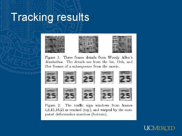
Tracking results

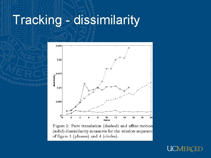
Tracking - dissimilarity

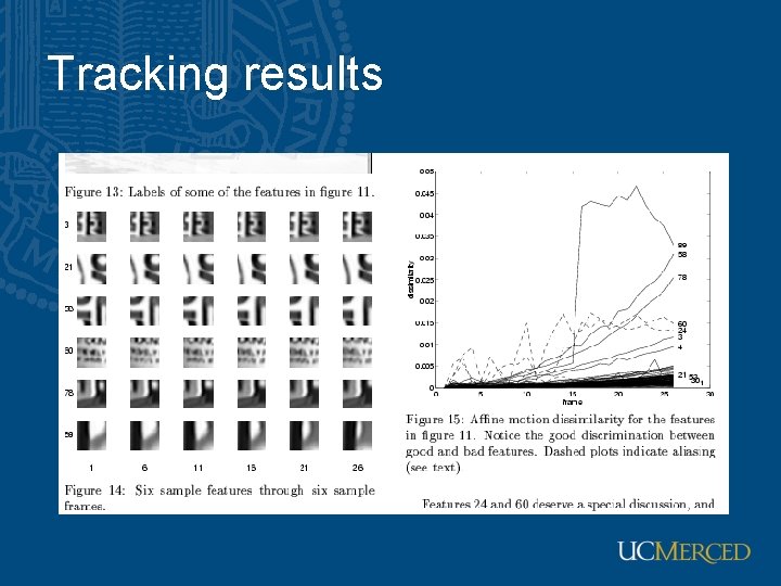
Tracking results

Correlation window size • Small windows lead to more false matches • Large windows are better this way, but… – Neighboring flow vectors will be more correlated (since the template windows have more in common) – Flow resolution also lower (same reason) – More expensive to compute • Small windows are good for local search: more detailed and less smooth (noisy? ) • Large windows good for global search: less detailed and smoother

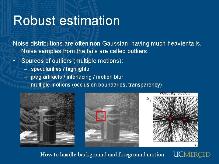
Robust estimation Noise distributions are often non-Gaussian, having much heavier tails. Noise samples from the tails are called outliers. • Sources of outliers (multiple motions): – specularities / highlights – jpeg artifacts / interlacing / motion blur – multiple motions (occlusion boundaries, transparency) u 2 velocity space + + u 1 How to handle background and foreground motion

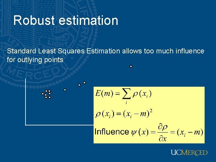
Robust estimation Standard Least Squares Estimation allows too much influence for outlying points

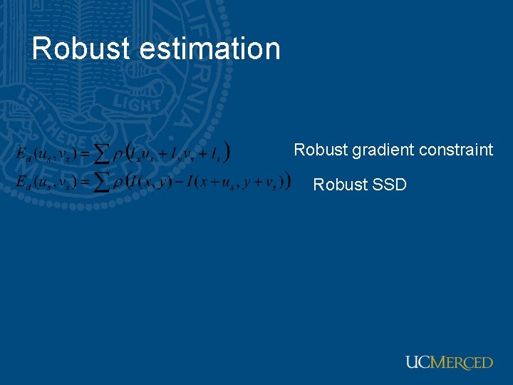
Robust estimation Robust gradient constraint Robust SSD

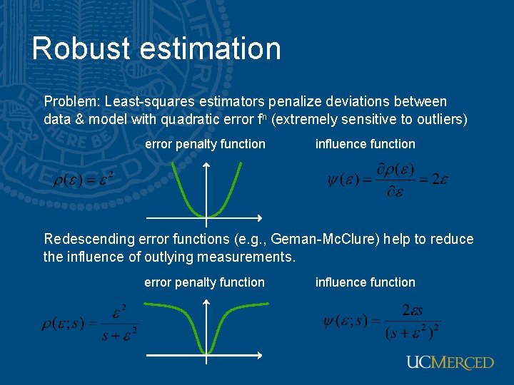
Robust estimation Problem: Least-squares estimators penalize deviations between data & model with quadratic error fn (extremely sensitive to outliers) error penalty function influence function Redescending error functions (e. g. , Geman-Mc. Clure) help to reduce the influence of outlying measurements. error penalty function influence function

Performance evaluation • See Baker et al. “A Database and Evaluation Methodology for Optical Flow”, ICCV 2007 • Algorithms: • Pyramid LK: Open. CV-based implementation of Lucas -Kanade on a Gaussian pyramid • Black and Anandan: Author’s implementation • Bruhn et al. : Our implementation • Media. Player. TM: Code used for video frame-rate upsampling in Microsoft Media. Player • Zitnick et al. : Author’s implementation

Performance evaluation • Difficulty: Data substantially more challenging than Yosemite • Diversity: Substantial variation in difficulty across the various datasets • Motion GT vs Interpolation: Best algorithms for one are not the best for the other • Comparison with Stereo: Performance of existing flow algorithms appears weak

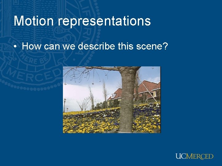
Motion representations • How can we describe this scene?

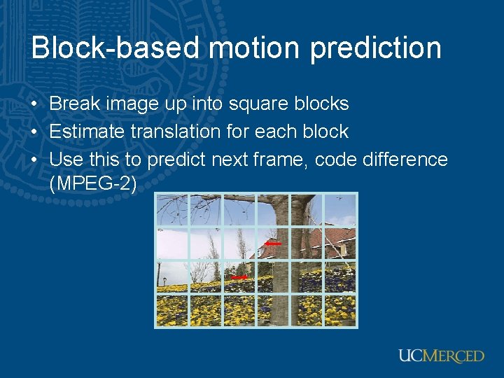
Block-based motion prediction • Break image up into square blocks • Estimate translation for each block • Use this to predict next frame, code difference (MPEG-2)

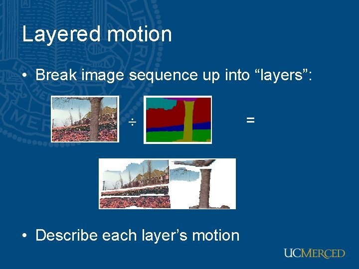
Layered motion • Break image sequence up into “layers”: • Describe each layer’s motion =

Layered motion • • Advantages: can represent occlusions / disocclusions each layer’s motion can be smooth video segmentation for semantic processing Difficulties: how do we determine the correct number? how do we assign pixels? how do we model the motion?

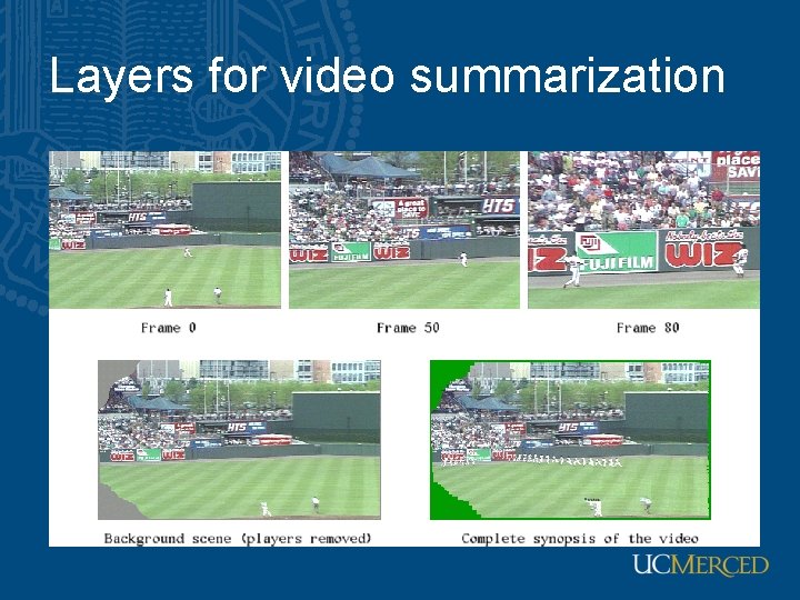
Layers for video summarization

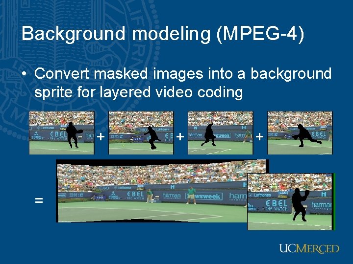
Background modeling (MPEG-4) • Convert masked images into a background sprite for layered video coding + = + + +

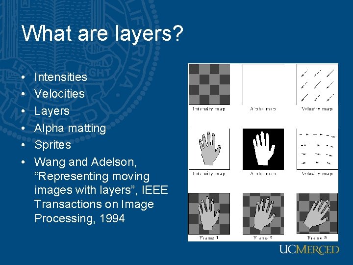
What are layers? • • • Intensities Velocities Layers Alpha matting Sprites Wang and Adelson, “Representing moving images with layers”, IEEE Transactions on Image Processing, 1994

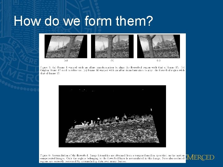
How do we form them?

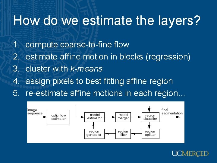
How do we estimate the layers? 1. 2. 3. 4. 5. compute coarse-to-fine flow estimate affine motion in blocks (regression) cluster with k-means assign pixels to best fitting affine region re-estimate affine motions in each region…

Layer synthesis • For each layer: • • stabilize the sequence with the affine motion compute median value at each pixel • Determine occlusion relationships

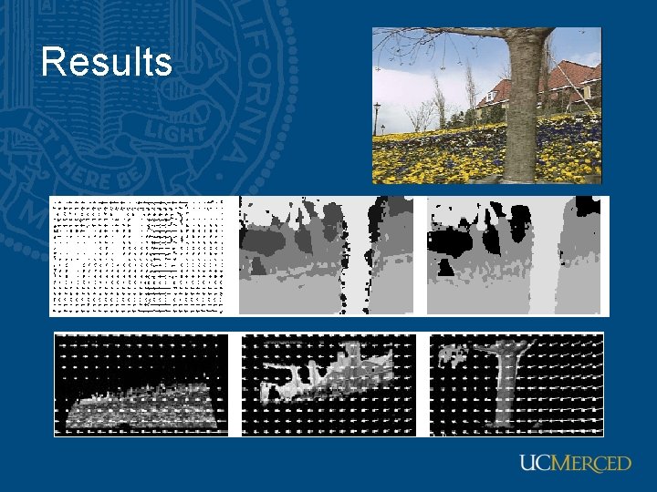
Results

Applications • • Motion analysis Video coding Morphing Video denoising Video stabilization Medical image registration Frame interpolation