EECS 274 Computer Vision Pyramid and Texture Filter

EECS 274 Computer Vision Pyramid and Texture

Filter, pyramid and texture • • • Frequency domain Fourier transform Gaussian pyramid Wavelets Texture • Reading: FP Chapters 8 and 9, S Chapters 3 and 4

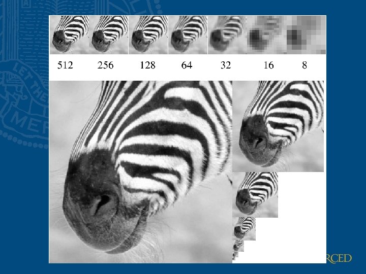
Scaled representations • Big bars (resp. spots, hands, etc. ) and little bars are both interesting – Stripes and hairs, say • Inefficient to detect big bars with big filters – And there is superfluous detail in the filter kernel • Alternative: – Apply filters of fixed size to images of different sizes – Typically, a collection of images whose edge length changes by a factor of 2 (or root 2) – This is a pyramid (or Gaussian pyramid) by visual analogy

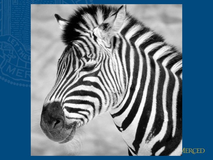
A bar in the big images is a hair on the zebra’s nose; in smaller images, a stripe; in the smallest, the animal’s nose

Gaussian pre-filtering G 1/8 G 1/4 Gaussian 1/2 Solution: filter the image, then subsample • Filter size should double for each ½ size reduction. Why?

Subsampling with Gaussian pre-filtering Gaussian 1/2 G 1/4 Solution: filter the image, then subsample • Filter size should double for each ½ size reduction. Why? • How can we speed this up? G 1/8

Compare with. . . 1/2 1/4 Why does this look so crufty? (2 x zoom) 1/8 (4 x zoom)

Aliasing • Can’t shrink an image by taking every second pixel • If we do, characteristic errors appear – In the next few slides – Typically, small phenomena look bigger; fast phenomena can look slower – Common phenomenon • Wagon wheels rolling the wrong way in movies • Checkerboards misrepresented in ray tracing • Striped shirts look funny on colour television

Resample the checkerboard by taking one sample at each circle. In the case of the top left board, new representation is reasonable. Top right also yields a reasonable representation. Bottom left is all black (dubious) and bottom right has checks that are too big. Sampling scheme is crucially related to frequency

Constructing a pyramid by taking every second pixel leads to layers that badly misrepresent the top layer

Open questions • What causes the tendency of differentiation to emphasize noise? • In what precise respects are discrete images different from continuous images? • How do we avoid aliasing? • General thread: a language for fast changes --- The Fourier Transform

The Fourier transform • Represent function on a new basis – Think of functions as vectors, with many components – We now apply a linear transformation to transform the basis • dot product with each basis element • In the expression, u and v select the basis element, so a function of x and y becomes a function of u and v • basis elements have the form • Measure amount of the sinusoid with given frequency and orientation in the signal

Fourier transform A: how much of a frequency component ϕ : where of a certain frequency is convole sinusoidal s(x) with a filter whose impulse repose h(x) another sinusoid of the same frequency but magnitude A and phase ϕ Tabulation of magnitude and phase response to each frequency

To get some sense of what basis elements look like, we plot a basis element --- or rather, its real part --as a function of x, y for some fixed u, v. We get a function that is constant when (ux+vy) is constant, e. g. , (u, v)=(1, 2) The magnitude of the vector (u, v) gives a frequency, and its direction gives an orientation. The function is a sinusoid with this frequency along the direction, and constant perpendicular to the direction. Spatial frequency component

Here u and v are larger than in the previous slide, (u, v)=(0, 0. 4)

And larger still. . .

Phase and magnitude • Fourier transform of a real function is complex – difficult to plot, visualize – instead, we can think of the phase and magnitude of the transform • Phase is the phase of the complex transform • Magnitude is the magnitude of the complex transform • Curious fact – all natural images have about the same magnitude transform – hence, phase seems to matter, but magnitude largely doesn’t • Demonstration – Take two pictures, swap the phase transforms, compute the inverse - what does the result look like?

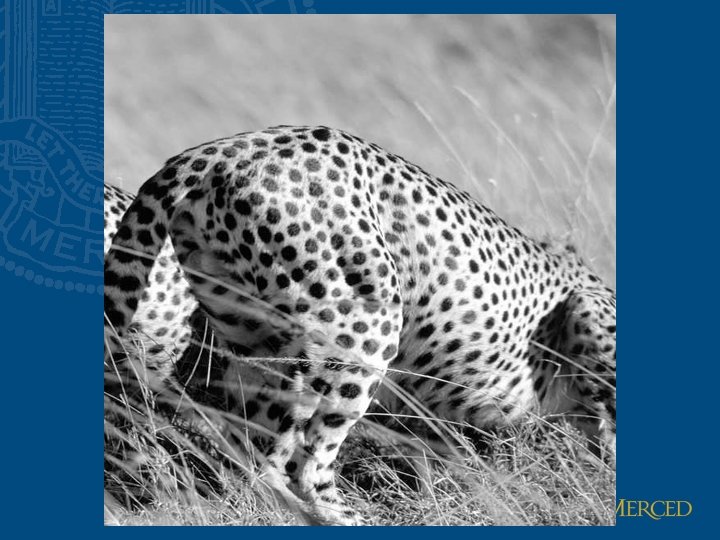
This is the magnitude transform of the cheetah pic

This is the phase transform of the cheetah pic

This is the magnitude transform of the zebra pic

This is the phase transform of the zebra pic

Reconstruction with zebra phase, cheetah magnitude Magnitude spctrum of an image is rather uninformative

Reconstruction with cheetah phase, zebra magnitude

Various Fourier Transform Pairs • Important facts – The Fourier transform is linear – There is an inverse FT – if you scale the function’s argument, then the transform’s argument scales the other way. This makes sense --- if you multiply a function’s argument by a number that is larger than one, you are stretching the function, so that high frequencies go to low frequencies – The FT of a Gaussian is a Gaussian. • The convolution theorem – The Fourier transform of the convolution of two functions is the product of their Fourier transforms – The inverse Fourier transform of the product of two Fourier transforms is the convolution of the two inverse Fourier transforms • There’s a table in the book.

Sampling in 1 D takes a continuous function and replaces it with a vector of values, consisting of the function’s values at a set of sample points. We’ll assume that these sample points are on a regular grid, and can place one at each integer for convenience.

Sampling in 2 D does the same thing, only in 2 D. We’ll assume that these sample points are on a regular grid, and can place one at each integer point for convenience.

A continuous model for a sampled function • We want to be able to approximate integrals sensibly • Leads to – the delta function – the following model Zero everywhere except at integer points

The Fourier transform of a sampled signal F(u, v) is the Fourier transform of f(x, y)

Example • Transform of box filter is sinc. • Transform of Gaussian is Gaussian. (Trucco and Verri)

Fourier transform of the sampled signal consists of a sum of copies of the Fourier transform of the original signal, shifted with respect to each other by the sampling frequency. If the shifted copies do not overlap, the original signal can be reconstructed from the sampled signal. If they overlap, we cannot obtain a separate copy of the Fourier transform, and the signal is aliased

If they overlap, we cannot obtain a separate copy of the Fourier transform, and the signal is aliased Nyquist theorem: sampling rate must be at least two times the cut –off frequency for perfect reconstruction

Smoothing as low-pass filtering • The message of the FT is that high frequencies lead to trouble with sampling. • Solution: suppress high frequencies before sampling – multiply the FT of the signal with something that suppresses high frequencies – or convolve with a low-pass filter • A filter whose FT is a box is bad, because the filter kernel has infinite support • Common solution: use a Gaussian – multiplying FT by Gaussian is equivalent to convolving image with Gaussian.

Sampling without smoothing. Top row shows the images, sampled at every second pixel to get the next; bottom row shows the magnitude spectrum of these images. substantial aliasing

Sampling with smoothing (small σ). Top row shows the images. We get the next image by smoothing the image with a Gaussian with σ=1 pixel, then sampling at every second pixel to get the next; bottom row shows the magnitude spectrum of these images. reducing aliasing Low pass filter suppresses high frequency components with less aliasing

Sampling with smoothing (large σ). Top row shows the images. We get the next image by smoothing the image with a Gaussian with σ=2 pixels, then sampling at every second pixel to get the next; bottom row shows the magnitude spectrum of these images. lose details Large σ less aliasing, but with little detail Gaussian is not an ideal low-pass filter

Decimation and interpolation Decimation (downsampling): Use an “ideal” anti-aliasing filter h(n) In practice, use FIR (finite impulse response) filter Interpolation (upsampling): Use an “ideal” interpolation filter h(n) In practice, use FIR (finite impulse response) filter

Applications of scaled representations • Search for correspondence – look at coarse scales, then refine with finer scales, coarse-to-fine matching – 4 × 4, 16 × 16, …, 1024 × 1024 versions of images • Edge tracking – a “good” edge at a fine scale has parents at a coarser scale • Control of detail and computational cost in matching – e. g. finding stripes – terribly important in texture representation

The Gaussian pyramid • Smooth with Gaussians, because – a Gaussian*Gaussian=another Gaussian • Gaussian filter operates as a low-pass filter • Synthesis – smooth and sample • Analysis – take the top image Use 3 -tap FIR, h(n)=(1/4, 1/2, 1/4) in dowsampling and 3 -tap FIR, h(n)=(1/2, 1, 1/2) for interpolation

The Laplacian pyramid • Analysis – preserve difference between upsampled Gaussian pyramid level and Gaussian pyramid level – band pass filter - each level represents spatial frequencies (largely) unrepresented at other levels • Synthesis – reconstruct Gaussian pyramid, take top layer

Lo. G and Do. G (difference of Gaussian) is widely used as an approximation to Lo. G (Laplacian of Gaussian)

Laplacian pyramid Different levels represent different spatial frequencies

Stripes give stronger response at particular scales as each layer corresponds to the band-pass filter output

Filters in spatial frequency domain • Fourier transform of a Gaussian with std of σ is the a Gaussian with std of 1/ σ • It falls off quickly in frequency domain and operates as a low-pass filter • Convolving an image with Gaussian with small σ all but the highest frequencies are preserved • Convolving an image with Gaussian with large σ like an average of the image

Example use: Smoothing/Blurring • We want a smoothed function of f(x) • Let us use a Gaussian kernel • Then H(u) attenuates high frequencies in F(u) (Low-pass Filter)!

Band-pass filter and orientation selective operators Respond strongly to signals of particular range of spatial frequencies and orientations

Oriented pyramids • Laplacian pyramid is orientation independent • Apply an oriented filter to determine orientations at each layer – by clever filter design, we can simplify synthesis – this represents image information at a particular scale and orientation

Reprinted from “Shiftable Multi. Scale Transforms, ” by Simoncelli et al. , IEEE Transactions on Information Theory, 1992, copyright 1992, IEEE

Oriented pyramids analysis synthesis

Gabor filters • • • Similar to 2 D receptive fields Self similar Band-pass filter Good spatial locality Sensitive to orientation Each kernel is a product of a Gaussian envelope and a complex plane wave • Often use Gabor wavelets of m scaled and n orientations • Successfully used in iris recognition

Wavelets LL LH HL HH

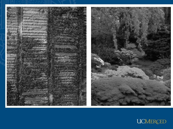
Texture • Key issue: representing texture – Texture based matching • little is known – Texture segmentation • key issue: representing texture – Texture synthesis • useful; also gives some insight into quality of representation – Shape from texture • cover superficially

Representing textures • Textures are made up of quite stylised subelements, repeated in meaningful ways • Representation: – find the subelements, and represent their statistics • But what are the subelements, and how do we find them? – recall normalized correlation – find subelements by applying filters, looking at the magnitude of the response • What filters? – experience suggests spots and oriented bars at a variety of different scales – details probably don’t matter • What statistics? – within reason, the more the merrier. – At least, mean and standard deviation – better, various conditional histograms.

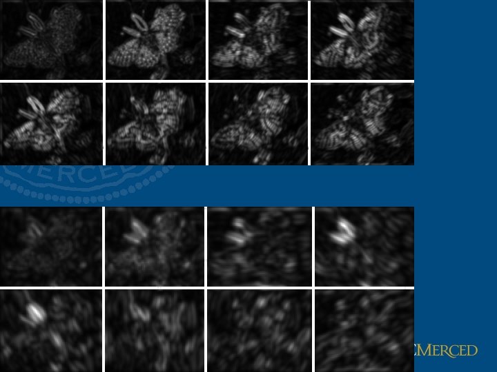
Spots and bars Two spots: • Weighted sum of 3 concentric Gaussians • Weighted sum of 2 concentric Gaussians Six bars: • Weighted sum of 3 oriented Gaussians Filter response at fine scale

Filter response at coarse scale

Gabor filters at different scales and spatial frequencies top row shows anti-symmetric (or odd) filters, bottom row the symmetric (or even) filters.

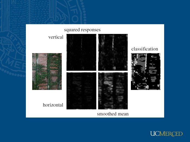
Final texture representation • Form an oriented pyramid (or equivalent set of responses to filters at different scales and orientations). • Square the output • Take statistics of responses – e. g. mean of each filter output (are there lots of spots) – std of each filter output – mean of one scale conditioned on other scale having a particular range of values (e. g. are the spots in straight rows? )

Texture synthesis • Use image as a source of probability model • Choose pixel values by matching neighborhood, then filling in • Matching process – look at pixel differences – count only synthesized pixels

Figure from Texture Synthesis by Non-parametric Sampling, A. Efros and T. K. Leung, Proc. Int. Conf. Computer Vision, 1999 copyright 1999, IEEE

FRAME • Model textures with filters, random fields, and maximum entropy • A set of filters is selected from a general filter bank to capture features of the texture and store the histograms • The maximum entropy principle is employed to derive a distribution p(I) • A stepwise algorithm is proposed to choose filters from a general filter bank. • The resulting model is a Markov random field (MRF) model, but with a much enriched vocabulary and hence much stronger descriptive ability than the previous MRF. • Gibbs sampler is adopted to synthesize texture images by drawing typical samples from P(I)

Variations • • Texture synthesis at multiple scales Texture synthesis on surfaces Texture synthesis by tiles “Analogous” texture synthesis

Dynamic texture • Model the underlying scene dynamics – Linear dynamic systems – Manifold learning • Used for synthesis • Video texture linear model nonlinear model