Dense Motion Estimation Reading Szeliski Chapter 8 Dense

Dense Motion Estimation Reading: Szeliski, Chapter 8

Dense Motion Estimation

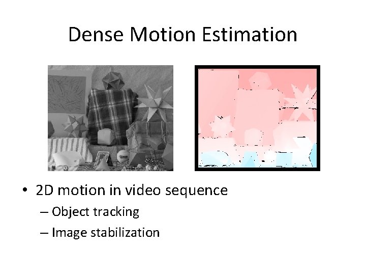
Dense Motion Estimation • 2 D motion in video sequence – Object tracking – Image stabilization

Motion Estimation • Error metric – Compare images • Search technique – Full search -- simple but slow – Hierarchical coarse-to-fine – Fourier transforms • Incremental methods • Optical flow – Multiple independent motions

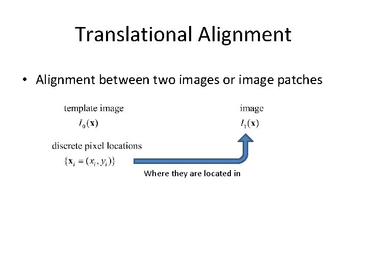
Translational Alignment • Alignment between two images or image patches Where they are located in

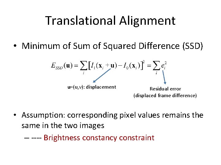
Translational Alignment • Minimum of Squared Difference (SSD) u=(u, v): displacement Residual error (displaced frame difference) • Assumption: corresponding pixel values remains the same in the two images – ---- Brightness constancy constraint

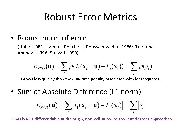
Robust Error Metrics • Robust norm of error (Huber 1981; Hampel, Ronchetti, Rousseeuw et al. 1986; Black and Anandan 1996; Stewart 1999) Grows less quickly than the quadratic penalty associated with least squares • Sum of Absolute Difference (L 1 norm) ESAD is NOT differentiable at the origin, not well suited to gradient descent approaches

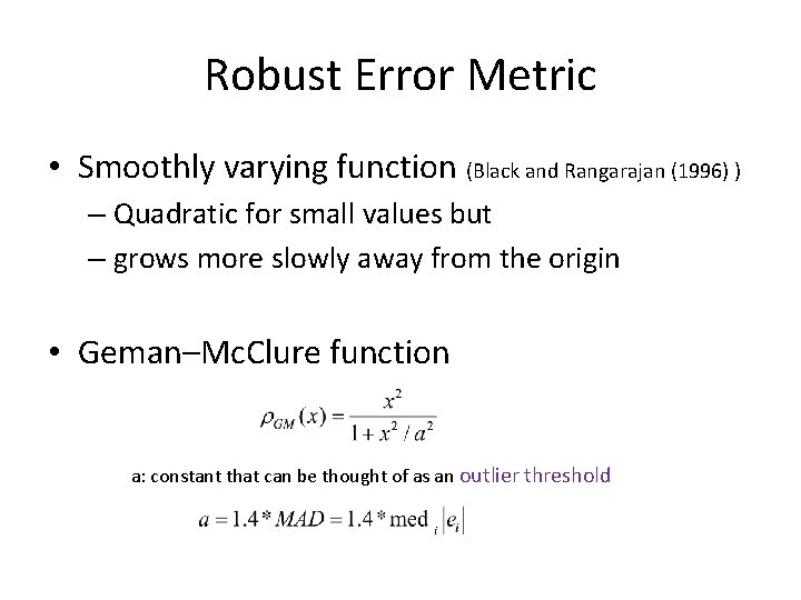
Robust Error Metric • Smoothly varying function (Black and Rangarajan (1996) ) – Quadratic for small values but – grows more slowly away from the origin • Geman–Mc. Clure function a: constant that can be thought of as an outlier threshold

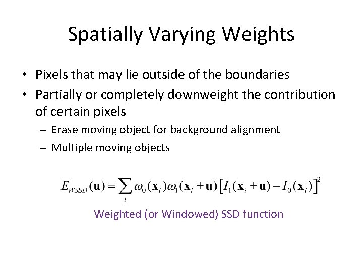
Spatially Varying Weights • Pixels that may lie outside of the boundaries • Partially or completely downweight the contribution of certain pixels – Erase moving object for background alignment – Multiple moving objects Weighted (or Windowed) SSD function

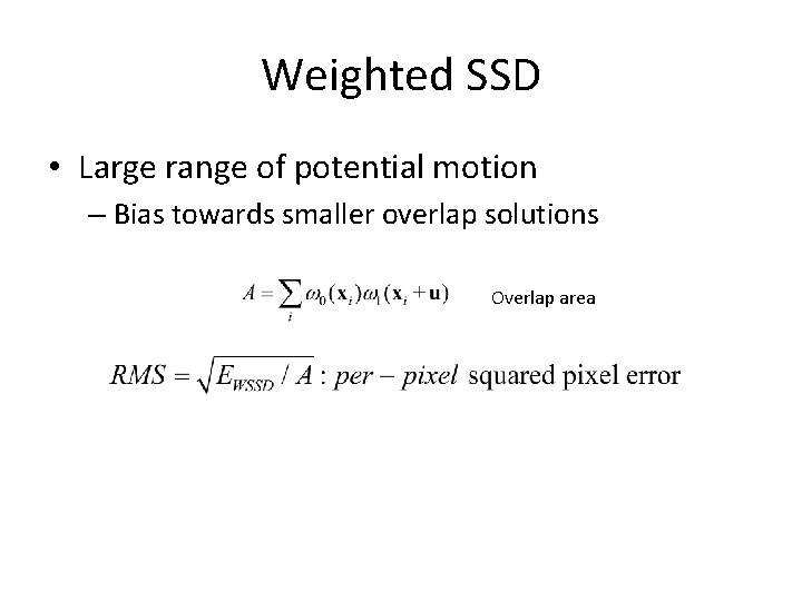
Weighted SSD • Large range of potential motion – Bias towards smaller overlap solutions Overlap area

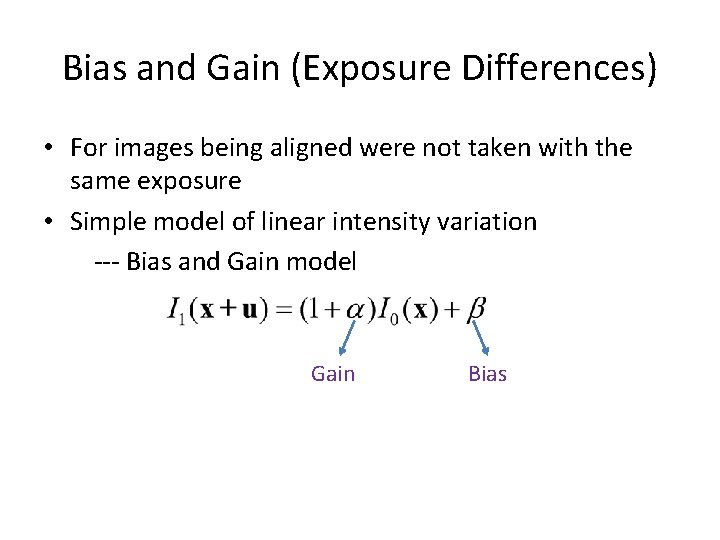
Bias and Gain (Exposure Differences) • For images being aligned were not taken with the same exposure • Simple model of linear intensity variation --- Bias and Gain model Gain Bias

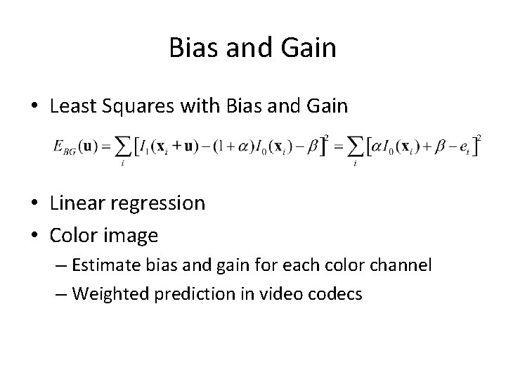
Bias and Gain • Least Squares with Bias and Gain • Linear regression • Color image – Estimate bias and gain for each color channel – Weighted prediction in video codecs

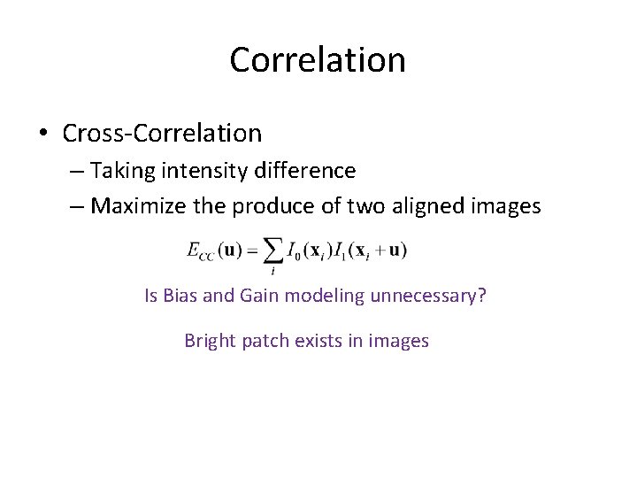
Correlation • Cross-Correlation – Taking intensity difference – Maximize the produce of two aligned images Is Bias and Gain modeling unnecessary? Bright patch exists in images

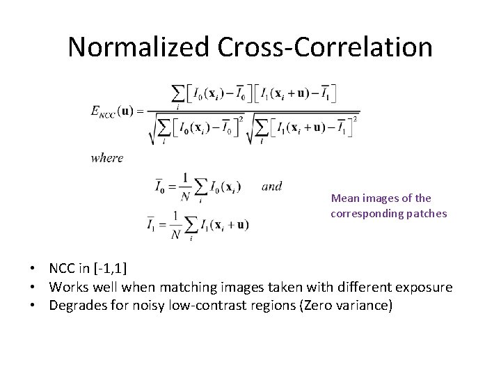
Normalized Cross-Correlation Mean images of the corresponding patches • NCC in [-1, 1] • Works well when matching images taken with different exposure • Degrades for noisy low-contrast regions (Zero variance)

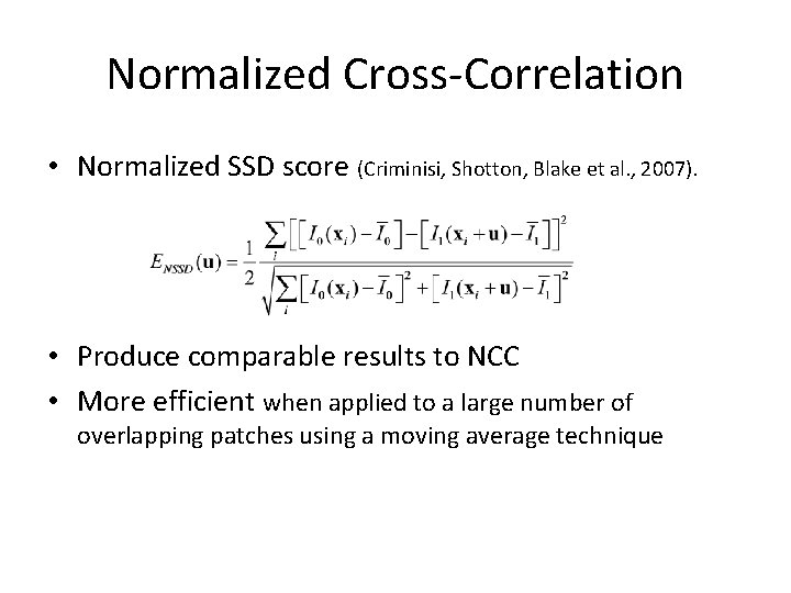
Normalized Cross-Correlation • Normalized SSD score (Criminisi, Shotton, Blake et al. , 2007). • Produce comparable results to NCC • More efficient when applied to a large number of overlapping patches using a moving average technique

Hierarchical Motion Estimation • How can we find its minimum? • Full search over some range of shifts – Often used for block matching in motion compensated video compression – Simple to implement but slow • To accelerate the search process – Hierarchical motion estimation

Hierarchical Motion Estimation • Steps – Construct image pyramid – At coarser levels, search over a smaller number of discrete pixels – Motion estimation at coarse level is used to initialize a smaller local search at the next finer level • Not guaranteed to produce the same results as a full search, but works almost as well and much faster

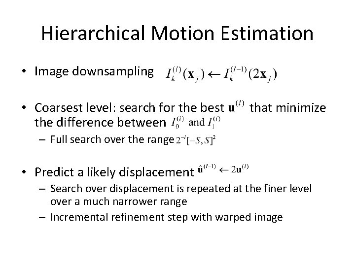
Hierarchical Motion Estimation • Image downsampling • Coarsest level: search for the best the difference between that minimize – Full search over the range • Predict a likely displacement – Search over displacement is repeated at the finer level over a much narrower range – Incremental refinement step with warped image

Incremental Refinement • Nearest pixel – integer pixel • Higher accuracy is required for stabilization or stitching • Sub-pixel estimates – Evaluate several values (u, v) around the best value – Interpolate the matching score to find the analytic minimum • Gradient descent on SSD energy function

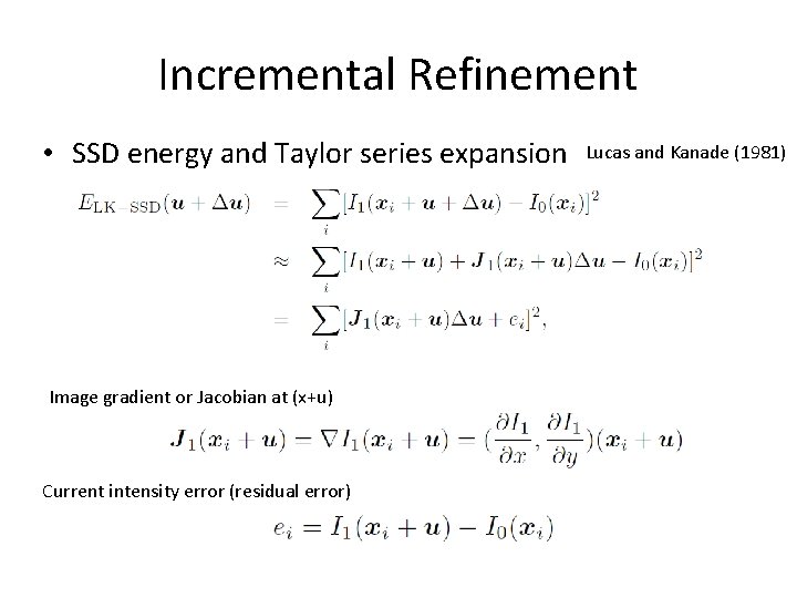
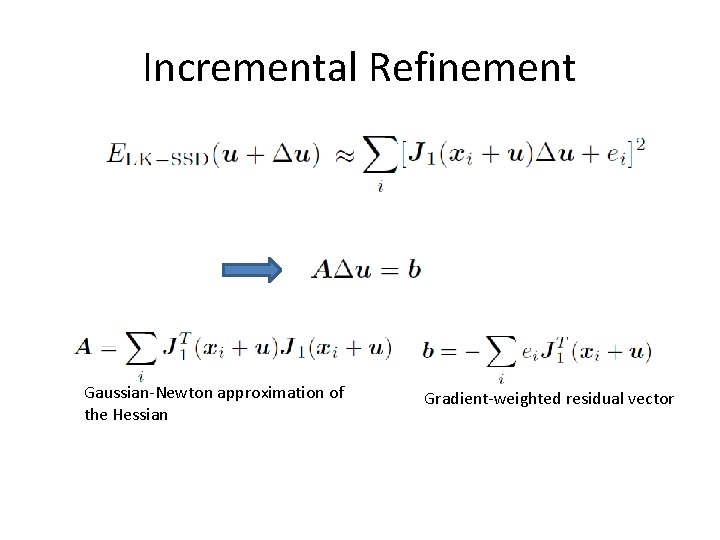
Incremental Refinement • SSD energy and Taylor series expansion Image gradient or Jacobian at (x+u) Current intensity error (residual error) Lucas and Kanade (1981)

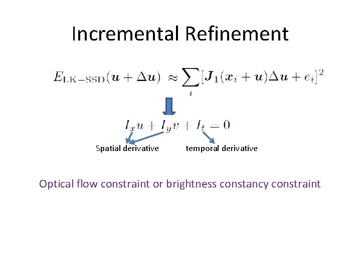
Incremental Refinement Spatial derivative temporal derivative Optical flow constraint or brightness constancy constraint

Incremental Refinement Gaussian-Newton approximation of the Hessian Gradient-weighted residual vector

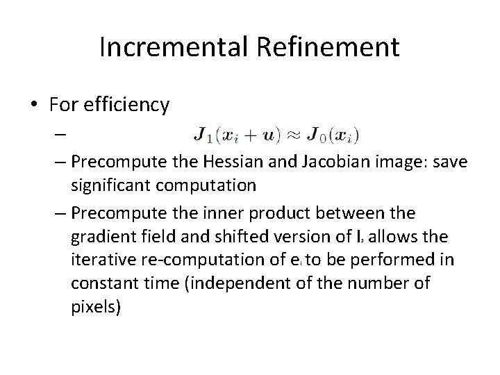
Incremental Refinement • For efficiency – – Precompute the Hessian and Jacobian image: save significant computation – Precompute the inner product between the gradient field and shifted version of I allows the iterative re-computation of e to be performed in constant time (independent of the number of pixels) 1 i

Incremental Refinement • Iterations – The effectiveness relies on the quality of Taylor series approximation – When far away from the true displacement (say, 1– 2 pixels), several iterations may be needed – It is possible to estimate a value for J_1 using a least squares fit to a series of larger displacements in order to increase the range of convergence (Jurie and Dhome 2002) or to “learn” a special-purpose recognizer for a given patch

Incremental Refinement • Stopping criterion – monitor the magnitude of the displacement correction |u| and to stop when it drops below a certain threshold (say, 1/10 of a pixel) • For larger motions – combine the incremental update rule with a hierarchical coarse-to-fine search strategy

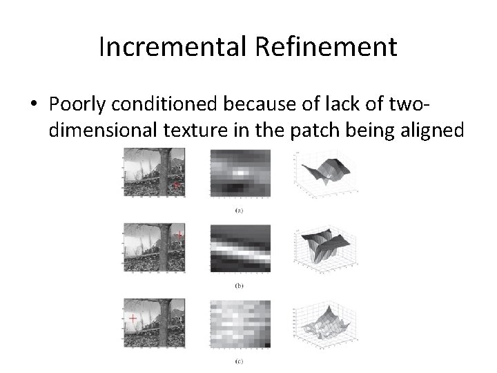
Incremental Refinement • Poorly conditioned because of lack of twodimensional texture in the patch being aligned

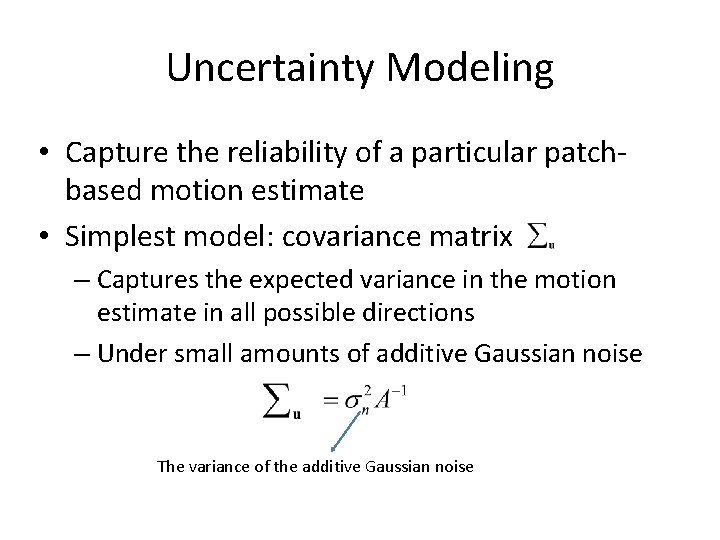
Uncertainty Modeling • Capture the reliability of a particular patchbased motion estimate • Simplest model: covariance matrix – Captures the expected variance in the motion estimate in all possible directions – Under small amounts of additive Gaussian noise The variance of the additive Gaussian noise

Uncertainty modeling • For larger amounts of noise, the linearization performed by the Lucas–Kanade algorithm is only approximate • The minimum and maximum eigenvalues of the Hessian A can now be interpreted as the (scaled) inverse variances in the least-certain and most-certain directions of motion.

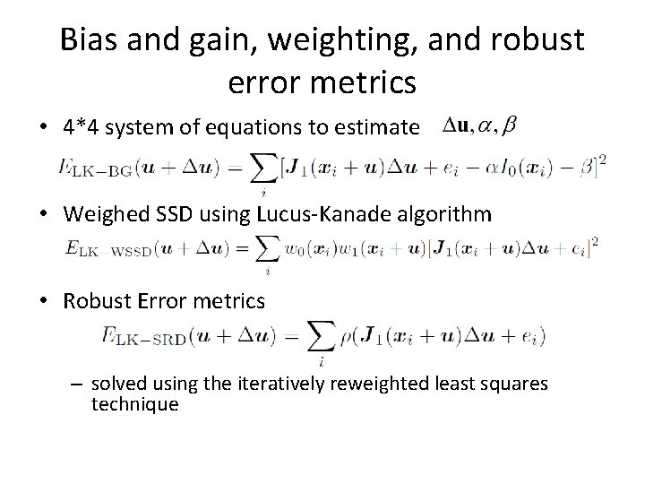
Bias and gain, weighting, and robust error metrics • 4*4 system of equations to estimate • Weighed SSD using Lucus-Kanade algorithm • Robust Error metrics – solved using the iteratively reweighted least squares technique

8. 2 Parametric Motion • More sophisticated motion models – Affine, has 4 unknowns – Full search over possible range is impractical – Lucas-Kanade algorithm parametric motion models (Lucas and Kanade 1981; Rehg and Witkin 1991; Fuh and Maragos 1991; Bergen, Anandan, Hanna et al. 1992; Shashua and Toelg 1997; Shashua and Wexler 2001; Baker and Matthews 2004).

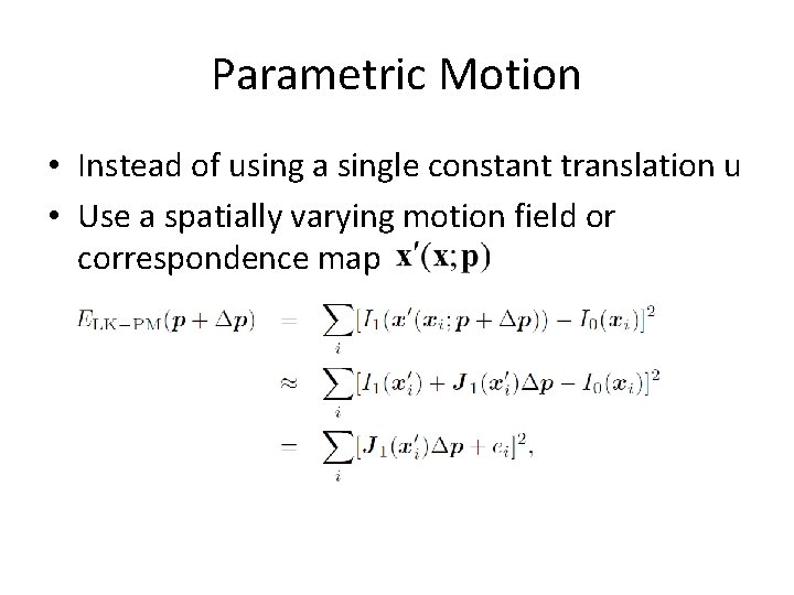
Parametric Motion • Instead of using a single constant translation u • Use a spatially varying motion field or correspondence map

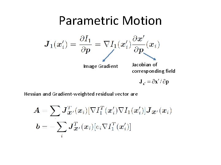
Parametric Motion Image Gradient Jacobian of corresponding field Hessian and Gradient-weighted residual vector are

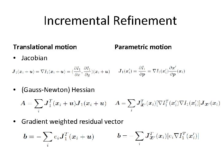
Incremental Refinement Translational motion Parametric motion • Jacobian • (Gauss-Newton) Hessian • Gradient weighted residual vector

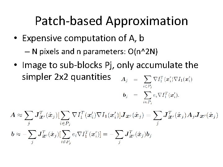
Patch-based Approximation • Expensive computation of A, b – N pixels and n parameters: O(n^2 N) • Image to sub-blocks Pj, only accumulate the simpler 2 x 2 quantities

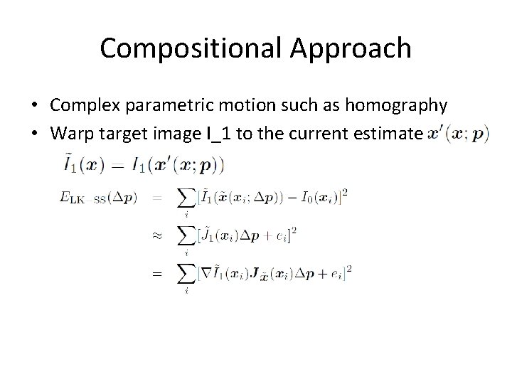
Compositional Approach • Complex parametric motion such as homography • Warp target image I_1 to the current estimate

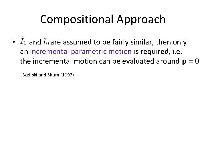
Compositional Approach • and are assumed to be fairly similar, then only an incremental parametric motion is required, i. e. the incremental motion can be evaluated around Szeliski and Shum (1997)

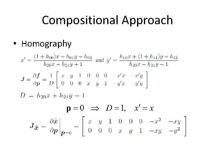
Compositional Approach • Homography

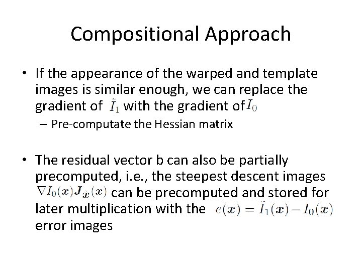
Compositional Approach • If the appearance of the warped and template images is similar enough, we can replace the gradient of with the gradient of – Pre-computate the Hessian matrix • The residual vector b can also be partially precomputed, i. e. , the steepest descent images can be precomputed and stored for later multiplication with the ea error images

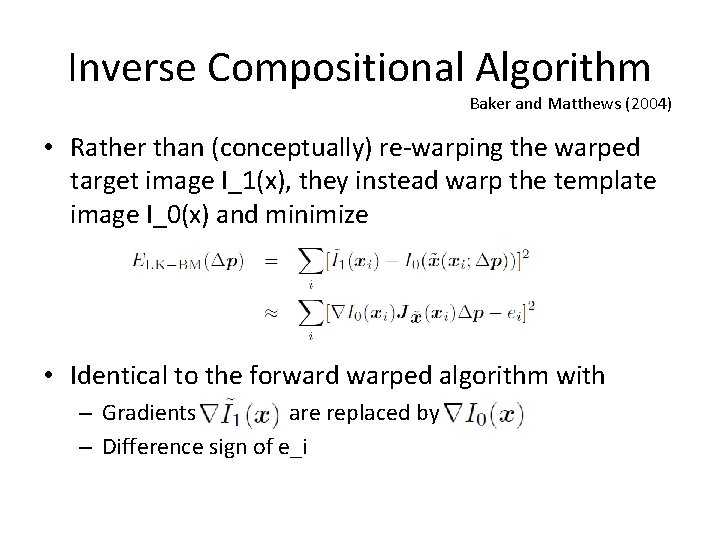
Inverse Compositional Algorithm Baker and Matthews (2004) • Rather than (conceptually) re-warping the warped target image I_1(x), they instead warp the template image I_0(x) and minimize • Identical to the forward warped algorithm with – Gradients are replaced by – Difference sign of e_i

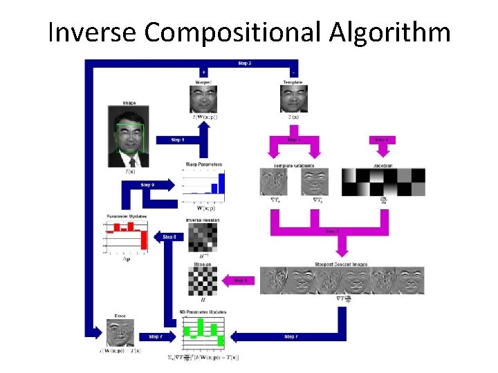
Inverse Compositional Algorithm

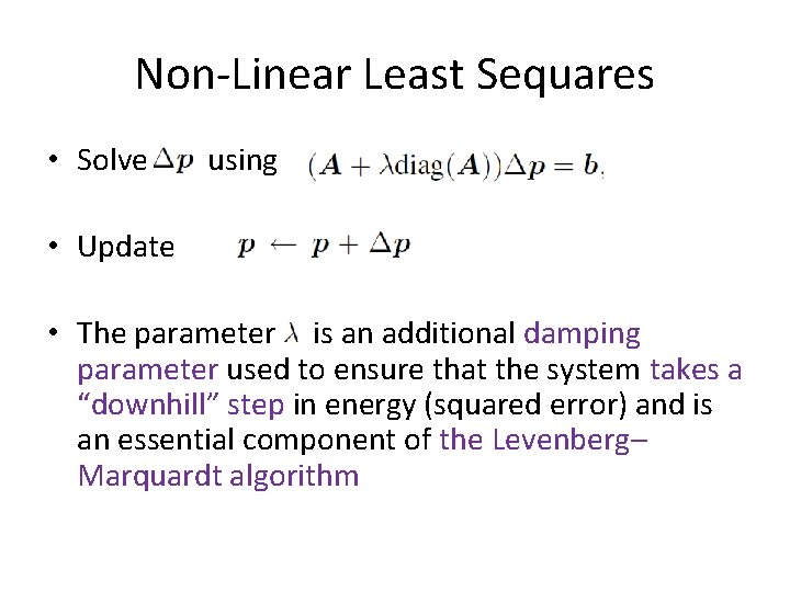
Non-Linear Least Sequares • Solve using • Update • The parameter is an additional damping parameter used to ensure that the system takes a “downhill” step in energy (squared error) and is an essential component of the Levenberg– Marquardt algorithm

8. 4 Optical Flow • Optical flow or optic flow is the pattern of apparent motion of objects, surfaces, and edges in a visual scene caused by the relative motion between an observer (an eye or a camera) and the scene. • The concept of optical flow was first studied in the 1940 s and ultimately published by American psychologist James J. Gibson[4] as part of his theory of affordance. • Optical flow techniques utilize this motion of the objects surfaces, and edges – motion detection, object segmentation, time-to-collision and focus of expansion calculations, motion compensated encoding, and stereo disparity measurement

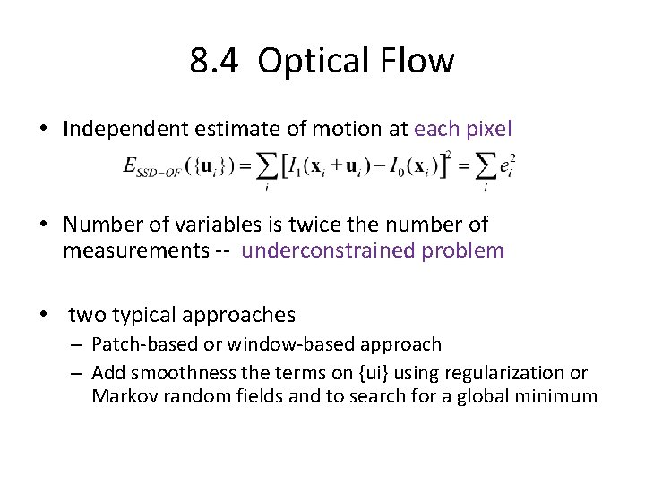
8. 4 Optical Flow • Independent estimate of motion at each pixel • Number of variables is twice the number of measurements -- underconstrained problem • two typical approaches – Patch-based or window-based approach – Add smoothness the terms on {ui} using regularization or Markov random fields and to search for a global minimum

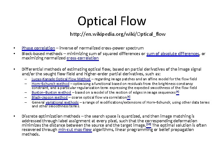
Optical Flow http: //en. wikipedia. org/wiki/Optical_flow • • Phase correlation – inverse of normalized cross-power spectrum Block-based methods – minimizing sum of squared differences or sum of absolute differences, or maximizing normalized cross-correlation • Differential methods of estimating optical flow, based on partial derivatives of the image signal and/or the sought flow field and higher-order partial derivatives, such as: – – – • Lucas–Kanade Optical Flow Method – regarding image patches and an affine model for the flow field Horn–Schunck method – optimizing a functional based on residuals from the brightness constancy constraint, and a particular regularization term expressing the expected smoothness of the flow field Buxton–Buxton method – based on a model of the motion of edges in image sequences [9] Black–Jepson method – coarse optical flow via correlation [6] General variational methods – a range of modifications/extensions of Horn–Schunck, using other data terms and other smoothness terms. Discrete optimization methods – the search space is quantized, and then image matching is addressed through label assignment at every pixel, such that the corresponding deformation minimizes the distance between the source and the target image. [10] The optimal solution is often recovered through min-cut max-flow algorithms, linear programming or belief propagation methods.

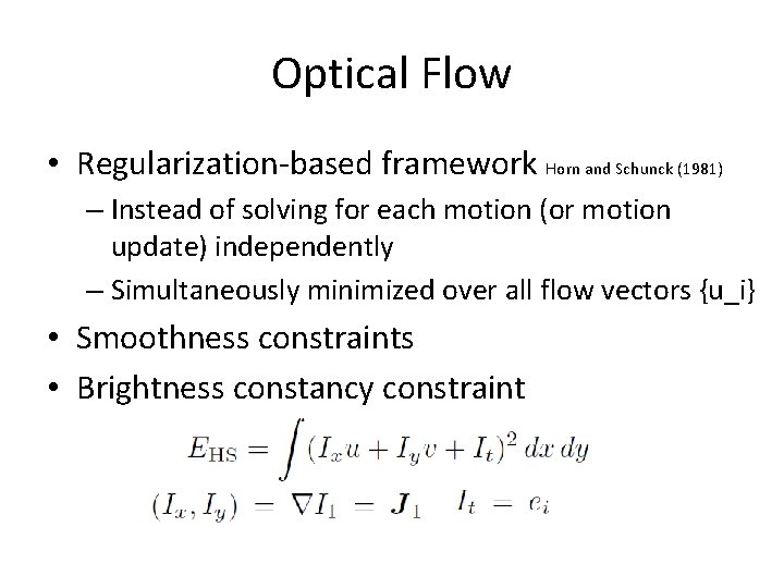
Optical Flow • Regularization-based framework Horn and Schunck (1981) – Instead of solving for each motion (or motion update) independently – Simultaneously minimized over all flow vectors {u_i} • Smoothness constraints • Brightness constancy constraint

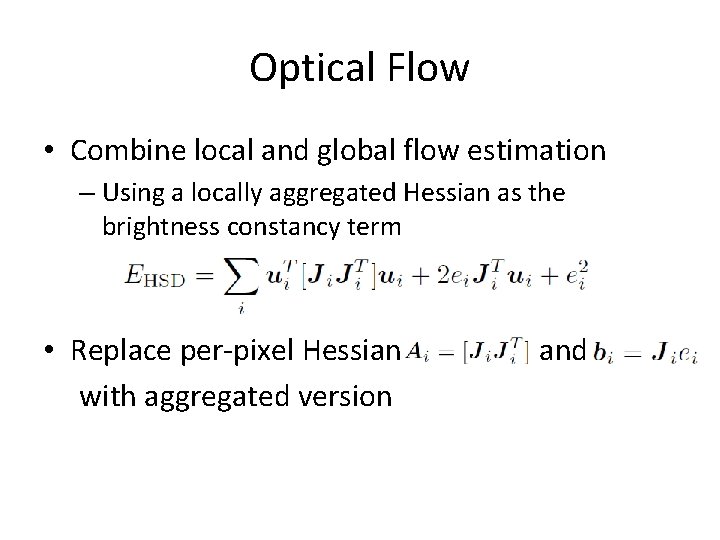
Optical Flow • Combine local and global flow estimation – Using a locally aggregated Hessian as the brightness constancy term • Replace per-pixel Hessian with aggregated version and

Optical Flow • Combine global (parametric) and local motion models • Estimate either per-image or per-segment affine motion models combined with per-pixel residual corrections • Image brightness varying • Gradient descent and coarse-to-fine continuation methods to minimize the global energy function • Combinatorial optimization methods based on Markov random fields

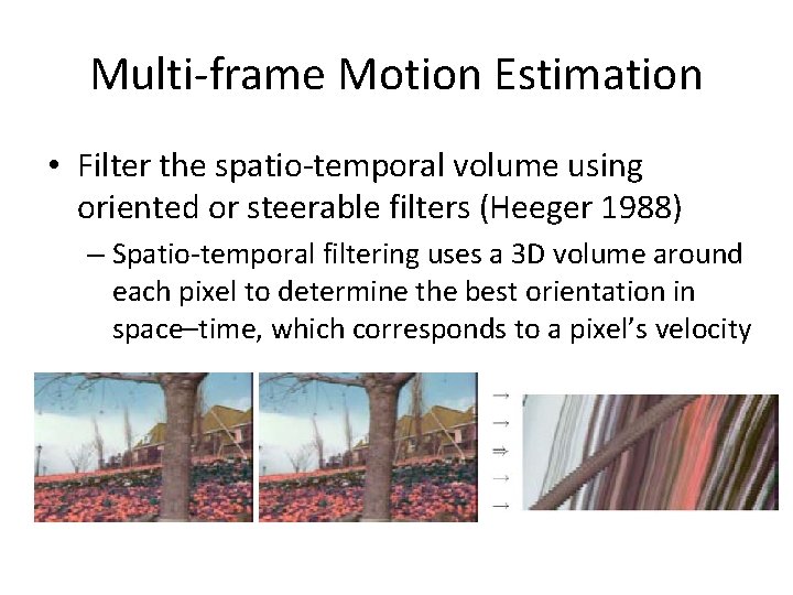
Multi-frame Motion Estimation • Filter the spatio-temporal volume using oriented or steerable filters (Heeger 1988) – Spatio-temporal filtering uses a 3 D volume around each pixel to determine the best orientation in space–time, which corresponds to a pixel’s velocity

Multi-frame Motion Estimation • Spatio-temporal filters have moderately large extents, which severely degrades the quality of their estimates near motion discontinuities • An alternative to full spatio-temporal filtering is to estimate more local spatio-temporal derivatives and use them inside a global optimization framework to fill in textureless regions (Bruhn, Weickert, and Schnorr 2005; Govindu 2006).

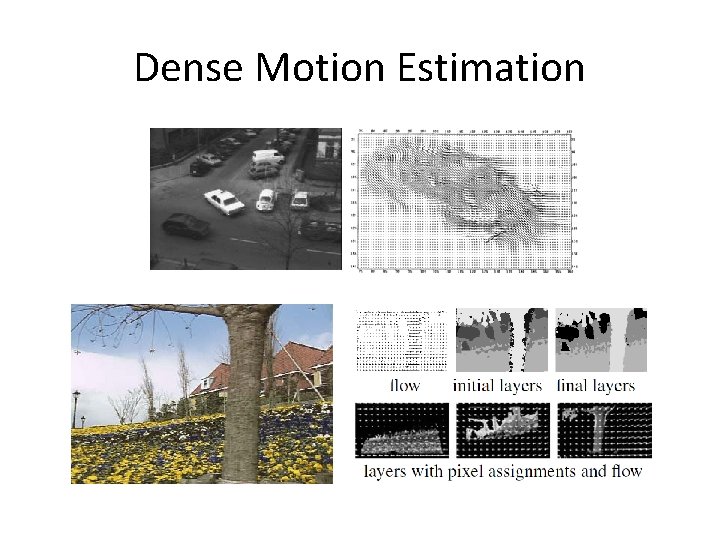
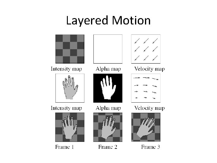
8. 5 Layered Motion • Global smoothness? Local neighborhood constraints? • Visual motion is caused by the movement of a number of objects at different depths – Pixels are grouped into appropriate objects or layers – The pixel motions can be described more succintly and estimated more reliably

Layered Motion

Layered Motion • Compact representation • Exploit the information available in multiple video frames • Accurately modeling the appearance of pixels near motion discontinuities • Image-based rendering • Object-level video editing

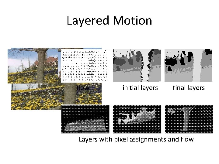
Layered Motion Wang and Adelson (1994) • How to compute layered representation of a video? – Estimate affine motion models over a collection of nonoverlapping patches – Cluster the estimates using K-means – Alternate between • Assigning pixels to layers • Recomputing the motion estimates for each layer – Construct layers • by warping and merging the various layer pieces from all frames together • median filter(shape composite layers that are robust to small intensity variations, infer occlusion between layers)

Layered Motion flow initial layers final layers Layers with pixel assignments and flow

Layered Motion Weiss and Adelson (1996) • Probabilistic mixture model to – infer both the optimal number of layers and – the per-pixel layer assignments • Per-layer affine motion smooth regularized per-pixel motion (Weiss 1997) – Better handle curved layers

Layered Motion • Distinction between motion estimating and layer assignments • Later estimating the layer colors • Generalized to account for real-world rigid motion scenes Baker, Szeliski, and Anandan (1998)

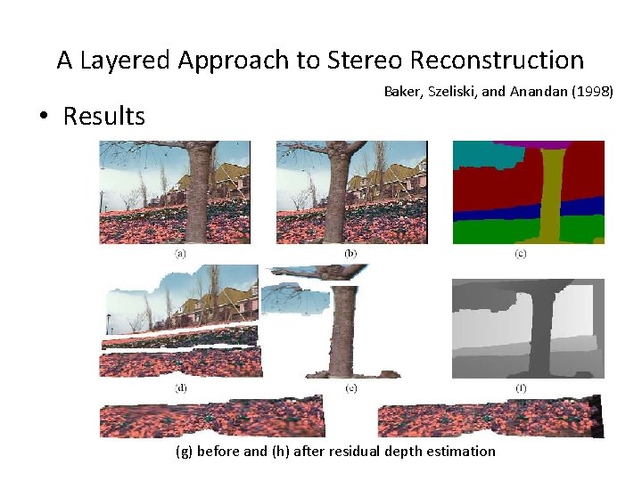
A Layered Approach to Stereo Reconstruction Baker, Szeliski, and Anandan (1998) • Motion of each frame – Described using a 3 D camera model • Motion of each layer – Described using 3 D plane equation + – Per-pixel residual depth offsets • Initial layers estimation – Similar to [Wang and Adelson, 1994] – Affine motion homography • Final model refinement – Jointly re-optimize the layer pixel color and opacity and depth, plane, and motion parameters – By minimizing the discrepency between the re 0 synthesized and observed motion sequence

A Layered Approach to Stereo Reconstruction • Results Baker, Szeliski, and Anandan (1998) (g) before and (h) after residual depth estimation

A Layered Approach to Stereo Reconstruction Baker, Szeliski, and Anandan (1998) • Motion boundaries and layer assignments are much crisper • Individual layer color values are also shaper – because of per-pixel depth offsets • Require a rough initial assignment • Improvement [Torr, Szeliski, and Anandan, 2001] – Automated Bayesian techniques for • initializing the system and • Determining the optimal number of layers

Layered Motion • Active research area – Sawhney and Ayer 1996; – Jojic and Frey 2001; – Xiao and Shah 2005; – Kumar, Torr, and Zisserman 2008; – Thayananthan, Iwasaki, and Cipolla 2008; – Schoenemann and Cremers 2008). • Alternate between segmentation and estimation of optical flow

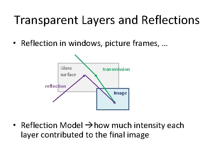
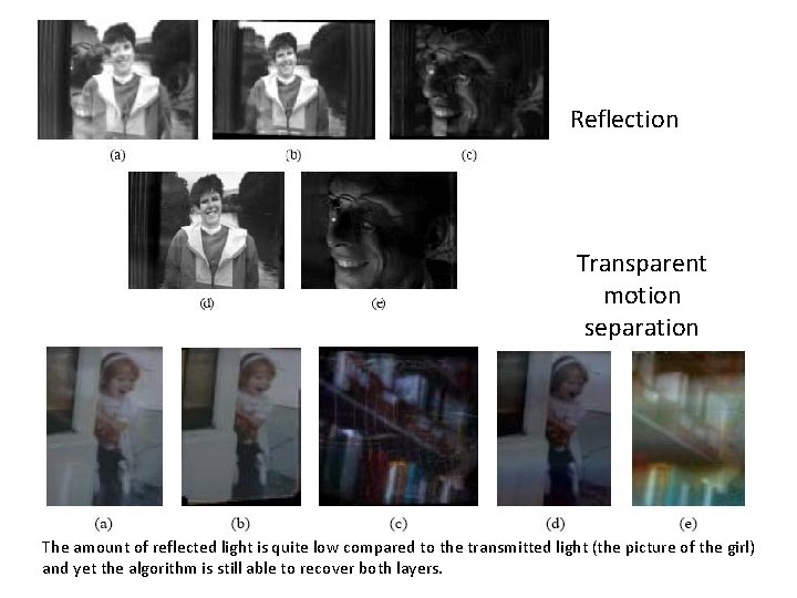
Transparent Layers and Reflections • Reflection in windows, picture frames, … Glass surface transmission reflection Image • Reflection Model how much intensity each layer contributed to the final image

Reflection Transparent motion separation The amount of reflected light is quite low compared to the transmitted light (the picture of the girl) and yet the algorithm is still able to recover both layers.

Transparent Layers and Reflections • If the motions of individual layers are known Recovery of individual layers Constrained Least Squares Positive layers • Suffer from low-frequency ambiguities – Especially, the layers lacks dark pixels – The motion is uni-directional

Transparent Layers and Reflections Szeliski, Avidan, and Anandan (2000) • Simultaneous estimation of motion and layer – Alternating between • Robustly computing the motion layers • Making conservative estimates of the layer intensities – Final motion and layer • Polished using gradient descent on joint constrained least squares • Parametric motion models – Only valid for planar reflectors & scenes with shallow depth – More extensions: Swaminathan, Kang, Szeliski et al. 2002; Criminisi, Kang, Swaminathan et al. 2005, Tsin, Kang, and Szeliski 2006