EECS 274 Computer Vision Stereopsis Stereopsis Epipolar geometry

EECS 274 Computer Vision Stereopsis

Stereopsis • • Epipolar geometry Trifocal tensor Stereopsis: Fusion and Reconstruction Correlation-Based Fusion Multi-Scale Edge Matching Dynamic Programming Using Three or More Cameras Reading: FP Chapter 7, S Chapter 11

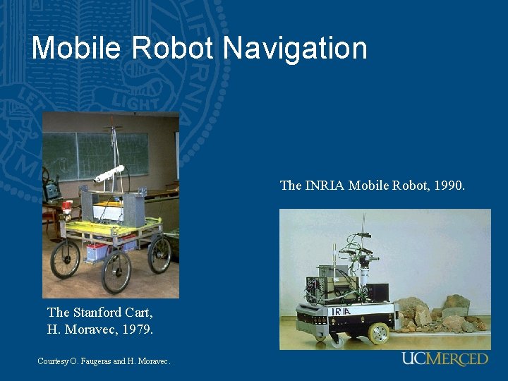
Mobile Robot Navigation The INRIA Mobile Robot, 1990. The Stanford Cart, H. Moravec, 1979. Courtesy O. Faugeras and H. Moravec.

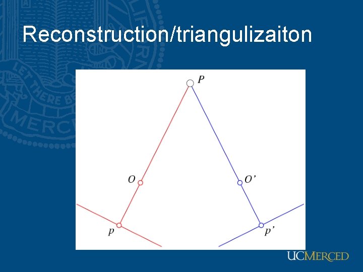
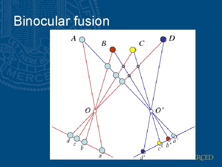
Stereo vision • Fusion: match points observed by two or more cameras • Reconstruction: find the pre-image of the matching points in 3 D world • Assume calibrated camera and essential matrix or trifocal tensors associated with 3 cameras are known

Reconstruction/triangulizaiton

Binocular fusion

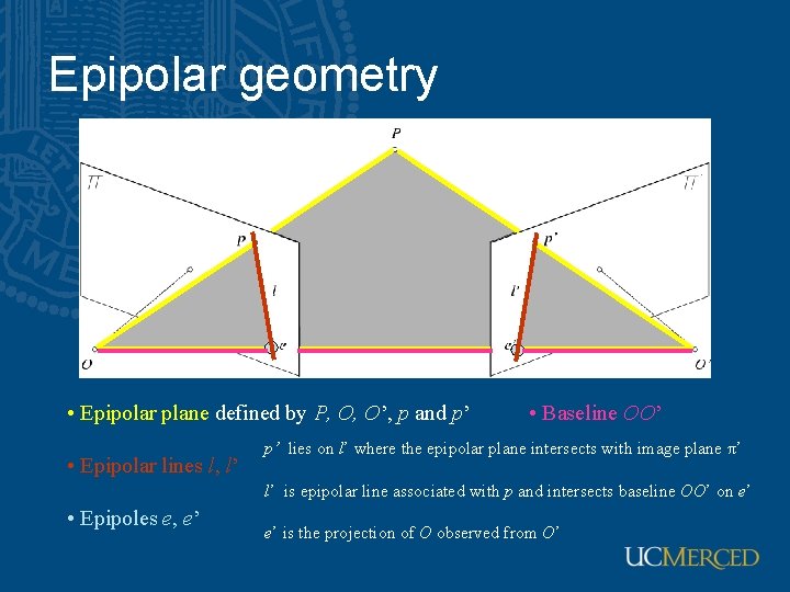
Epipolar geometry • Epipolar plane defined by P, O, O’, p and p’ • Epipolar lines l, l’ • Baseline OO’ p’ lies on l’ where the epipolar plane intersects with image plane π’ l’ is epipolar line associated with p and intersects baseline OO’ on e’ • Epipoles e, e’ e’ is the projection of O observed from O’

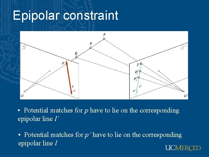
Epipolar constraint • Potential matches for p have to lie on the corresponding epipolar line l’ • Potential matches for p’ have to lie on the corresponding epipolar line l

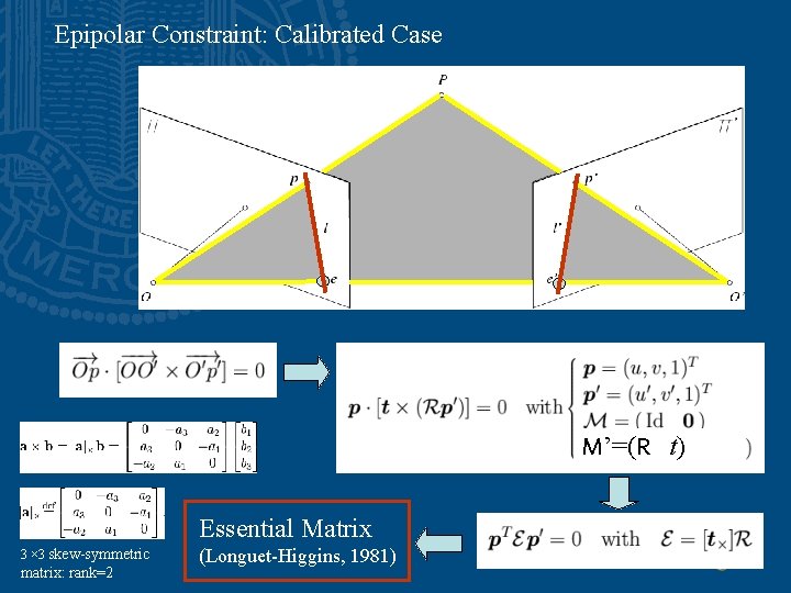
Epipolar Constraint: Calibrated Case M’=(R t) Essential Matrix 3 × 3 skew-symmetric matrix: rank=2 (Longuet-Higgins, 1981)

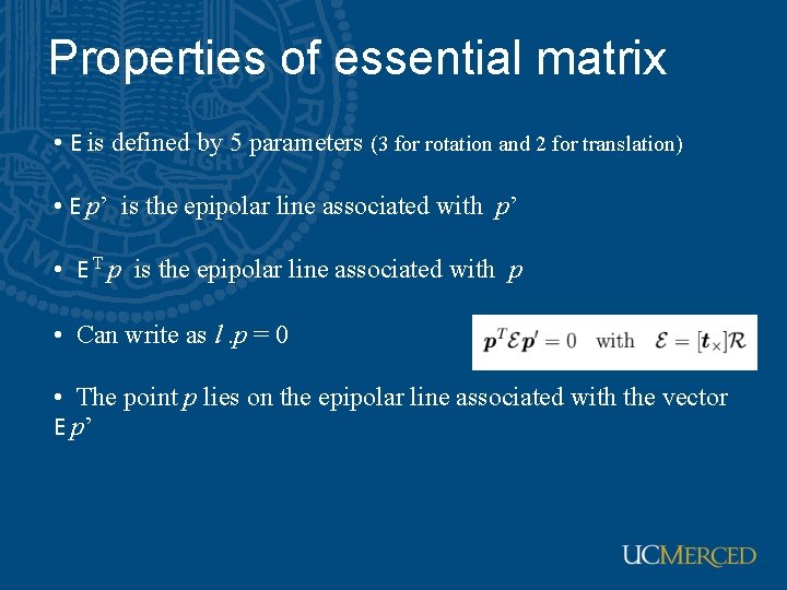
Properties of essential matrix • E is defined by 5 parameters (3 for rotation and 2 for translation) • E p’ is the epipolar line associated with p’ • E T p is the epipolar line associated with p • Can write as l. p = 0 • The point p lies on the epipolar line associated with the vector E p’

Properties of essential matrix (cont’d) • E e’=0 and ETe=0 (E e’=-RT[tx]e=0 ) • E is singular • E has two equal non-zero singular values (Huang and Faugeras, 1989)

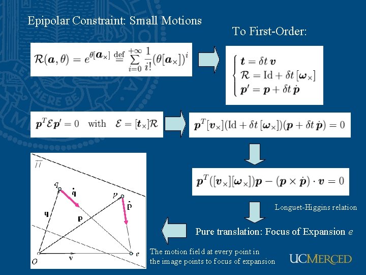
Epipolar Constraint: Small Motions To First-Order: Longuet-Higgins relation Pure translation: Focus of Expansion e The motion field at every point in the image points to focus of expansion

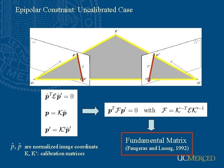
Epipolar Constraint: Uncalibrated Case are normalized image coordinate K, K’: calibration matrices Fundamental Matrix (Faugeras and Luong, 1992)

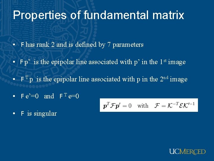
Properties of fundamental matrix • F has rank 2 and is defined by 7 parameters • F p’ is the epipolar line associated with p’ in the 1 st image • F T p is the epipolar line associated with p in the 2 nd image • F e’=0 and F T e=0 • F is singular

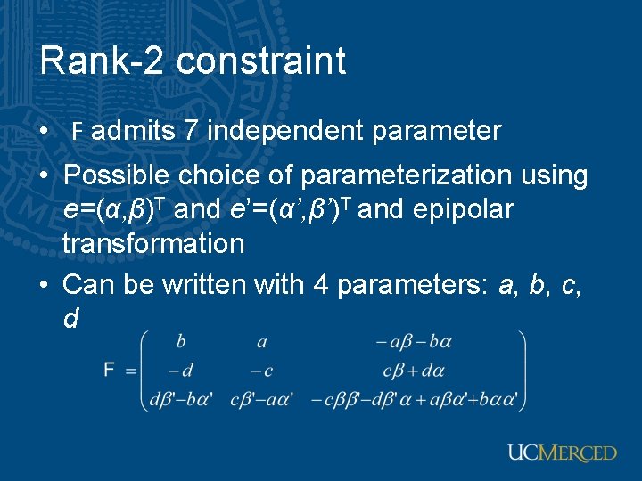
Rank-2 constraint • F admits 7 independent parameter • Possible choice of parameterization using e=(α, β)T and e’=(α’, β’)T and epipolar transformation • Can be written with 4 parameters: a, b, c, d

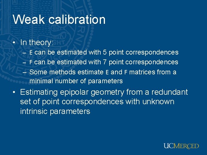
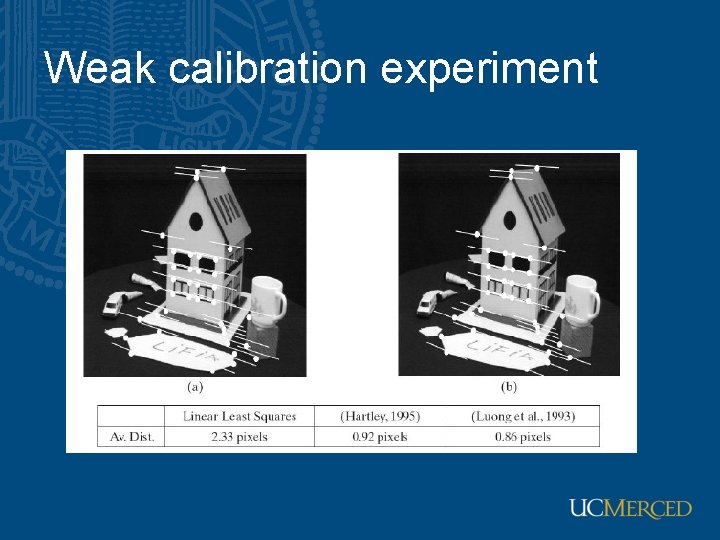
Weak calibration • In theory: – E can be estimated with 5 point correspondences – F can be estimated with 7 point correspondences – Some methods estimate E and F matrices from a minimal number of parameters • Estimating epipolar geometry from a redundant set of point correspondences with unknown intrinsic parameters

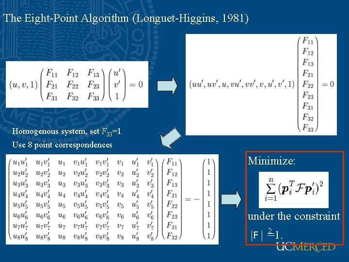
The Eight-Point Algorithm (Longuet-Higgins, 1981) Homogenous system, set F 33=1 Use 8 point correspondences Minimize: under the constraint 2 |F | =1.

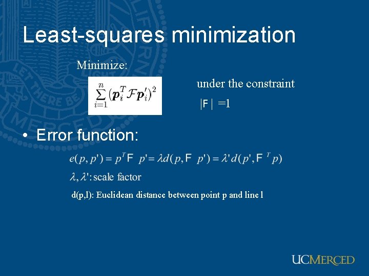
Least-squares minimization Minimize: under the constraint |F | =1 • Error function: d(p, l): Euclidean distance between point p and line l

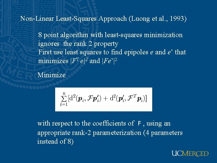
Non-Linear Least-Squares Approach (Luong et al. , 1993) 8 point algorithm with least-squares minimization ignores the rank 2 property First use least squares to find epipoles e and e’ that minimizes |FT e|2 and |Fe’|2 Minimize with respect to the coefficients of F , using an appropriate rank-2 parameterization (4 parameters instead of 8)

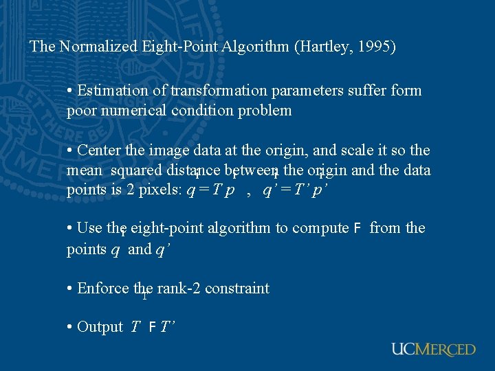
The Normalized Eight-Point Algorithm (Hartley, 1995) • Estimation of transformation parameters suffer form poor numerical condition problem • Center the image data at the origin, and scale it so the mean squared distance between the origin and the data i i points is 2 pixels: q = T p , q’ = T’ p’ • Use the eight-point algorithm to compute F from the i points q and q’ • Enforce the rank-2 constraint T • Output T F T’

Weak calibration experiment

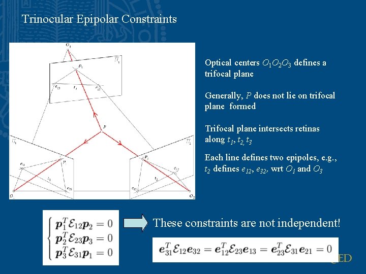
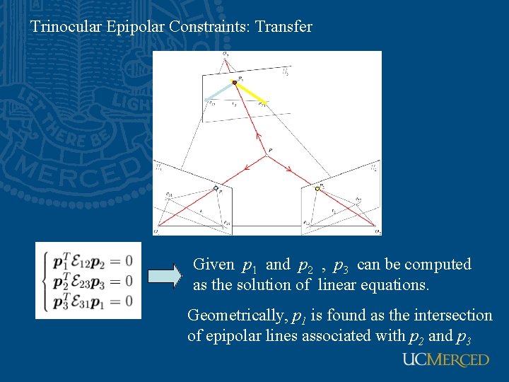
Trinocular Epipolar Constraints Optical centers O 1 O 2 O 3 defines a trifocal plane Generally, P does not lie on trifocal plane formed Trifocal plane intersects retinas along t 1, t 2, t 3 Each line defines two epipoles, e. g. , t 2 defines e 12, e 32, wrt O 1 and O 3 These constraints are not independent!

Trinocular Epipolar Constraints: Transfer Given p 1 and p 2 , p 3 can be computed as the solution of linear equations. Geometrically, p 1 is found as the intersection of epipolar lines associated with p 2 and p 3

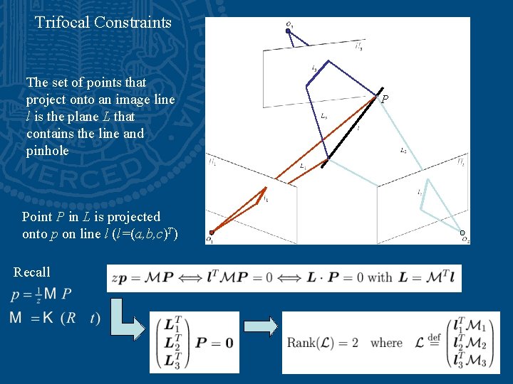
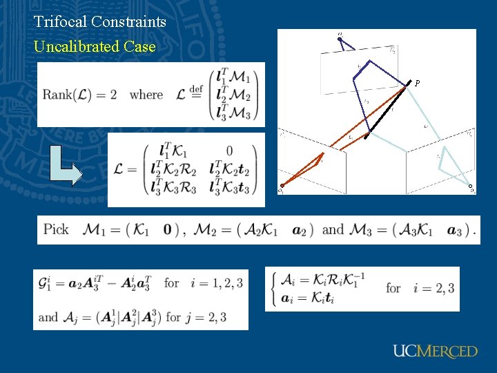
Trifocal Constraints The set of points that project onto an image line l is the plane L that contains the line and pinhole Point P in L is projected onto p on line l (l=(a, b, c)T) Recall P

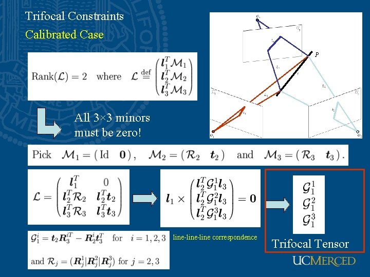
Trifocal Constraints Calibrated Case P All 3× 3 minors must be zero! line-line correspondence Trifocal Tensor

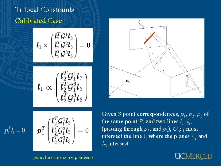
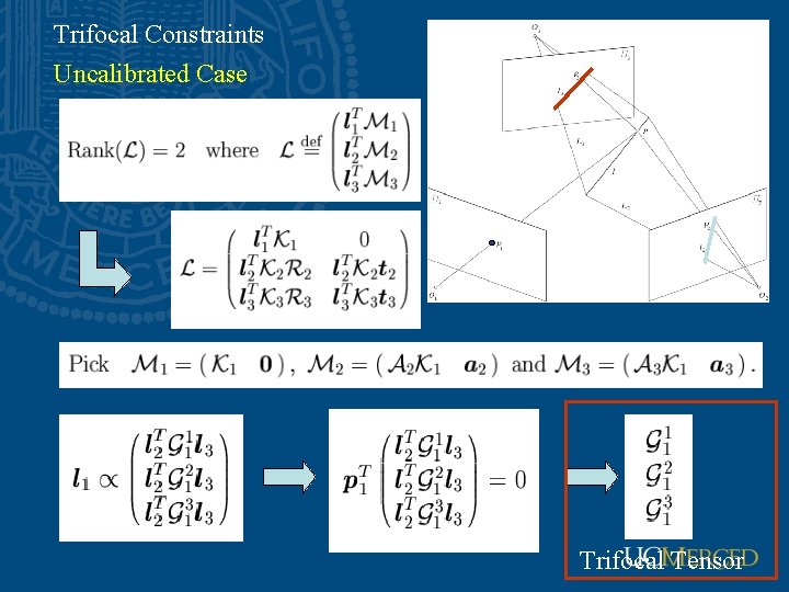
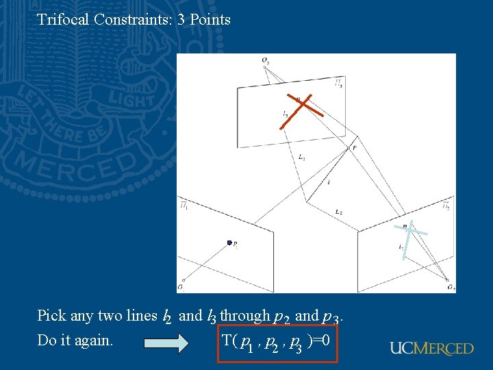
Trifocal Constraints Calibrated Case Given 3 point correspondences, p 1, p 2, p 3 of the same point P, and two lines l 2, l 3, (passing through p 2, and p 3), O 1 p 1 must intersect the line l, where the planes L 2 and L 3 intersect point-line correspondence

Trifocal Constraints Uncalibrated Case P

Trifocal Constraints Uncalibrated Case Trifocal Tensor

Trifocal Constraints: 3 Points Pick any two lines l and l through p and p . 2 3 Do it again. T( p 1 , p 2 , p )=0 3

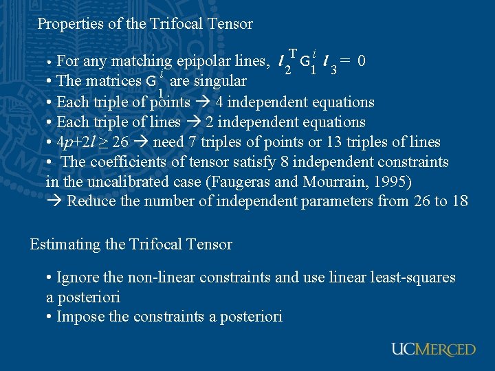
Properties of the Trifocal Tensor T i • For any matching epipolar lines, l G l = 0 2 1 3 i • The matrices G are singular 1 • Each triple of points 4 independent equations • Each triple of lines 2 independent equations • 4 p+2 l ≥ 26 need 7 triples of points or 13 triples of lines • The coefficients of tensor satisfy 8 independent constraints in the uncalibrated case (Faugeras and Mourrain, 1995) Reduce the number of independent parameters from 26 to 18 Estimating the Trifocal Tensor • Ignore the non-linear constraints and use linear least-squares a posteriori • Impose the constraints a posteriori

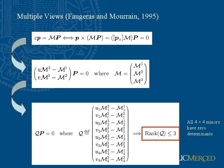
Multiple Views (Faugeras and Mourrain, 1995) All 4 × 4 minors have zero determinants

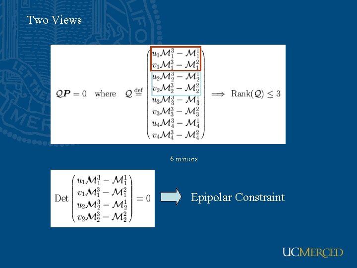
Two Views 6 minors Epipolar Constraint

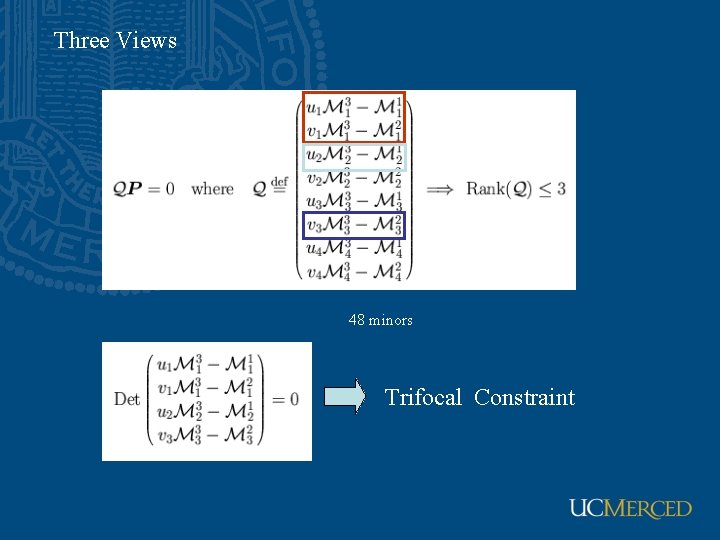
Three Views 48 minors Trifocal Constraint

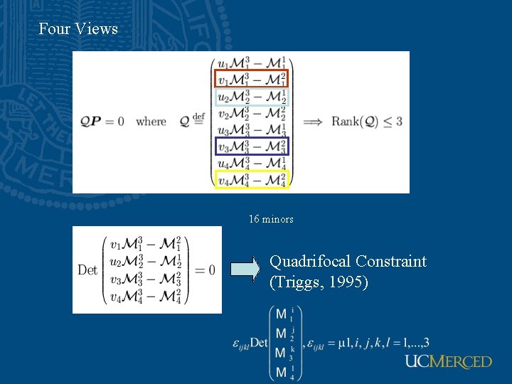
Four Views 16 minors Quadrifocal Constraint (Triggs, 1995)

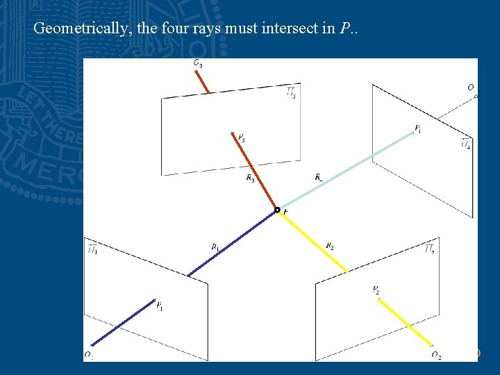
Geometrically, the four rays must intersect in P. .

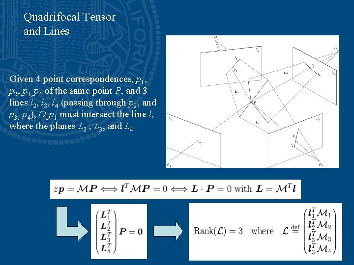
Quadrifocal Tensor and Lines Given 4 point correspondences, p 1, p 2, p 3, p 4 of the same point P, and 3 lines l 2, l 3, l 4 (passing through p 2, and p 3, p 4), O 1 p 1 must intersect the line l, where the planes L 2 , L 3, and L 4

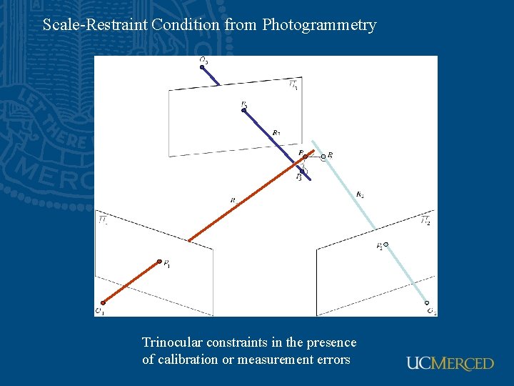
Scale-Restraint Condition from Photogrammetry Trinocular constraints in the presence of calibration or measurement errors

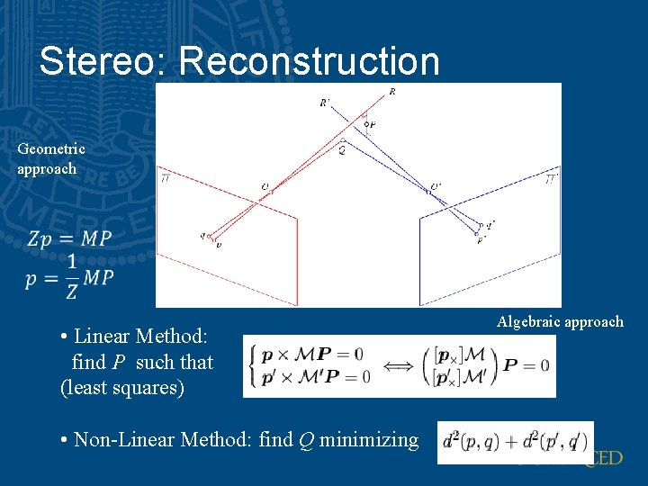
Stereo: Reconstruction Geometric approach • Linear Method: find P such that (least squares) • Non-Linear Method: find Q minimizing Algebraic approach

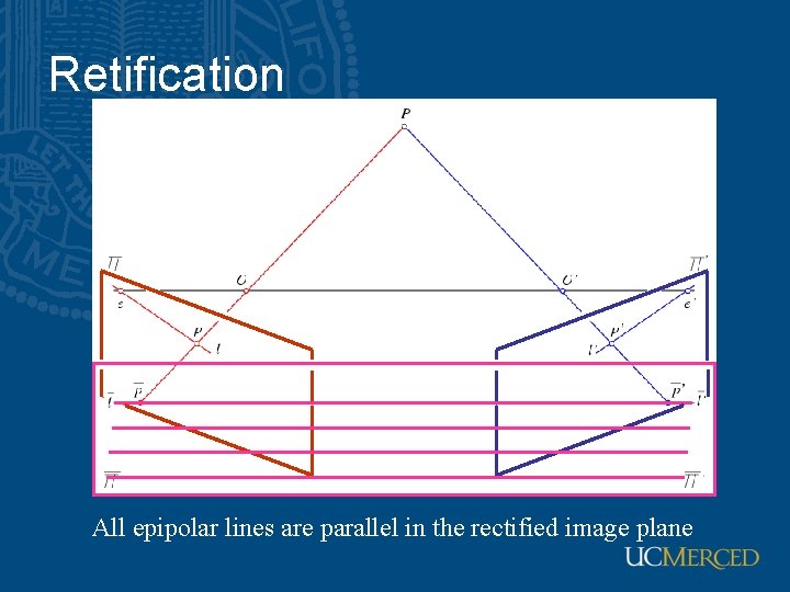
Retification All epipolar lines are parallel in the rectified image plane

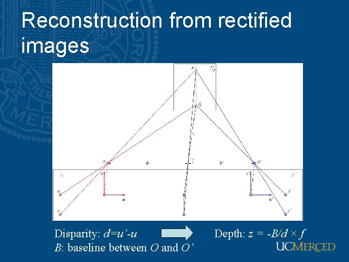
Reconstruction from rectified images Disparity: d=u’-u B: baseline between O and O’ Depth: z = -B/d × f

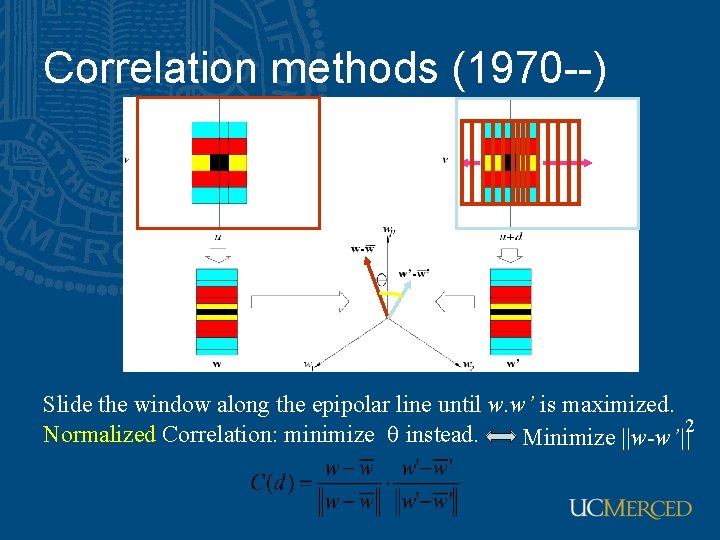
Correlation methods (1970 --) Slide the window along the epipolar line until w. w’ is maximized. 2 Normalized Correlation: minimize q instead. Minimize ||w-w’||

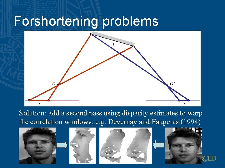
Forshortening problems Solution: add a second pass using disparity estimates to warp the correlation windows, e. g. Devernay and Faugeras (1994)

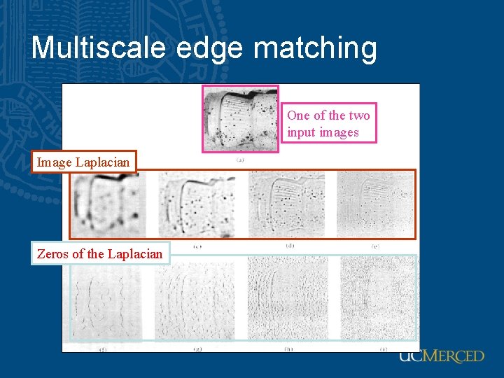
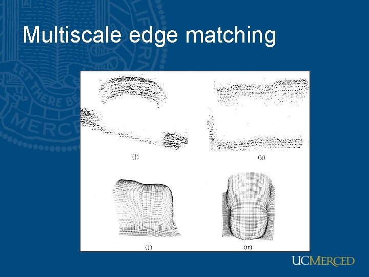
Multiscale edge matching [Marr, Poggio and Grimson, 1979 -81] • Edges are found by repeatedly smoothing the image and detecting the zero crossings of the second derivative (Laplacian) • Matches at coarse scales are used to offset the search for matches at fine scales (equivalent to eye movements)

Multiscale edge matching One of the two input images Image Laplacian Zeros of the Laplacian

Multiscale edge matching

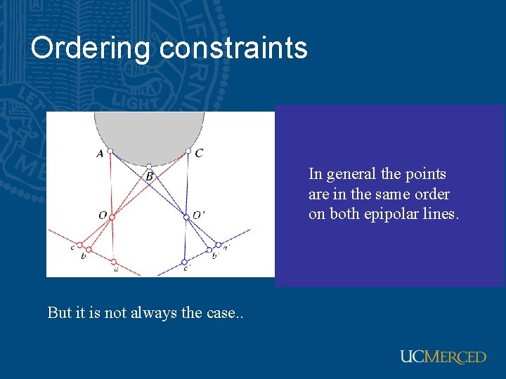
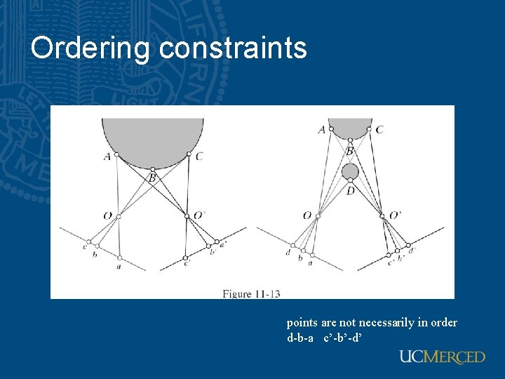
Ordering constraints In general the points are in the same order on both epipolar lines. But it is not always the case. .

Ordering constraints points are not necessarily in order d-b-a c’-b’-d’

Dynamic programming [Baker and Binford, 1981] Find the minimum-cost path going monotonically down and right from the top-left corner of the graph to its bottom-right corner. • Nodes = matched feature points (e. g. , edge points). • Arcs = matched intervals along the epipolar lines. • Arc cost = discrepancy between intervals.

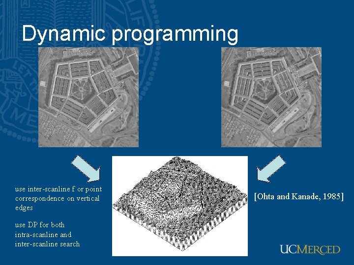
Dynamic programming use inter-scanline f or point correspondence on vertical edges use DP for both intra-scanline and inter-scanline search [Ohta and Kanade, 1985]

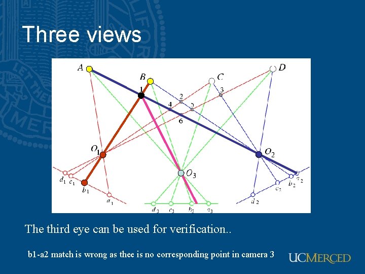
Three views The third eye can be used for verification. . b 1 -a 2 match is wrong as thee is no corresponding point in camera 3

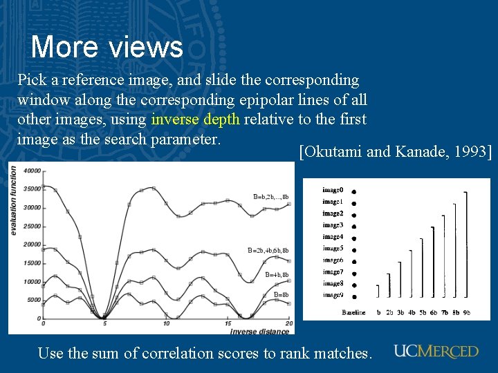
More views Pick a reference image, and slide the corresponding window along the corresponding epipolar lines of all other images, using inverse depth relative to the first image as the search parameter. [Okutami and Kanade, 1993] Use the sum of correlation scores to rank matches.

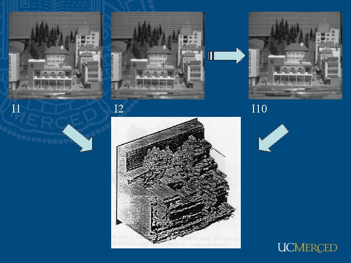
I 1 I 2 I 10

Correspondence • Extensive literature – Region based – Graph cut – Mutual information – Belief propagation – Conditional random field • Smooth surfaces

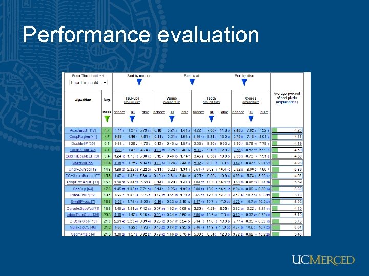
Middlebury stereo dataset • De facto data set with ground truth, code, and comprehensive performance evaluation • http: //vision. middlebury. edu/stereo/data/

Performance evaluation