EECS 274 Computer Vision Sources Shadows and Shading

EECS 274 Computer Vision Sources, Shadows, and Shading

Surface brightness • Depends on local surface properties (albedo), surface shape (normal), and illumination • Shading model: a model of how brightness of a surface is obtained • Can interpret pixel values to reconstruct its shape and albedo • Reading: FP Chapter 5, H Chapter 11

Radiometric properties of sources • How bright (or what color) are objects? • One more definition: Exitance of a light source is – the internally generated power (not reflected) radiated per unit area on the radiating surface • Similar to radiosity: a source can have both – radiosity, because it reflects – exitance, because it emits • Independent of its exit angle • Internally generated energy radiated per unit time, per unit area • But what aspects of the incoming radiance will we model? – Point, line, area source – Simple geometry

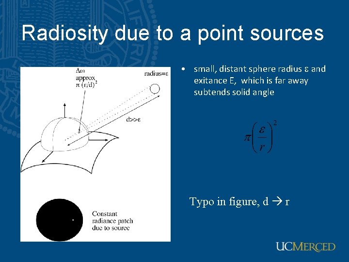
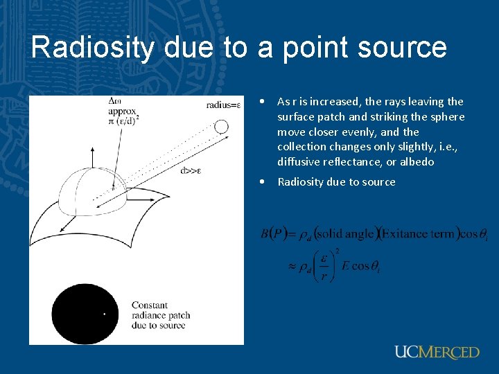
Radiosity due to a point sources • small, distant sphere radius e and exitance E, which is far away subtends solid angle Typo in figure, d r

Radiosity due to a point source • As r is increased, the rays leaving the surface patch and striking the sphere move closer evenly, and the collection changes only slightly, i. e. , diffusive reflectance, or albedo • Radiosity due to source

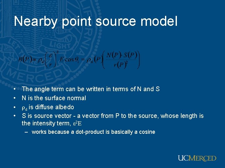
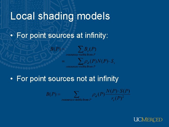
Nearby point source model • • The angle term can be written in terms of N and S N is the surface normal ρd is diffuse albedo S is source vector - a vector from P to the source, whose length is the intensity term, ε 2 E – works because a dot-product is basically a cosine

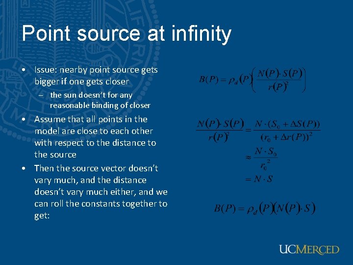
Point source at infinity • Issue: nearby point source gets bigger if one gets closer – the sun doesn’t for any reasonable binding of closer • Assume that all points in the model are close to each other with respect to the distance to the source • Then the source vector doesn’t vary much, and the distance doesn’t vary much either, and we can roll the constants together to get:

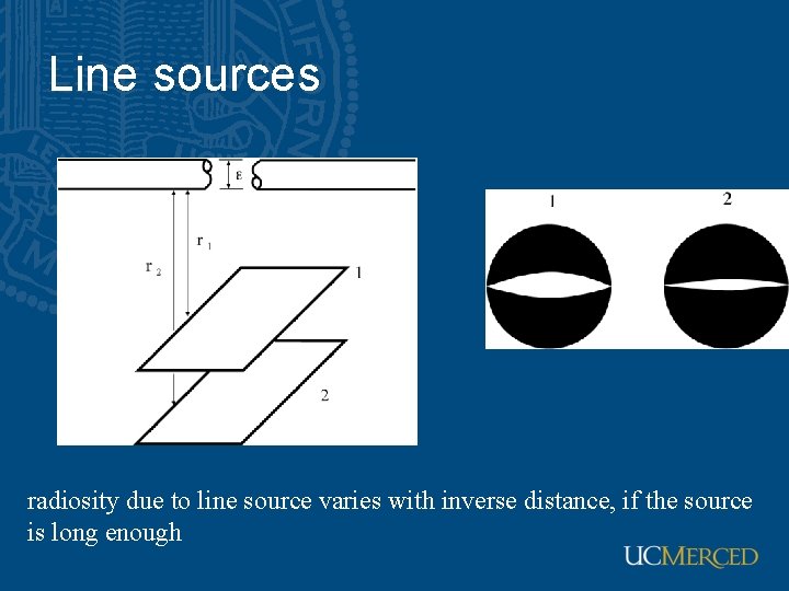
Line sources radiosity due to line source varies with inverse distance, if the source is long enough

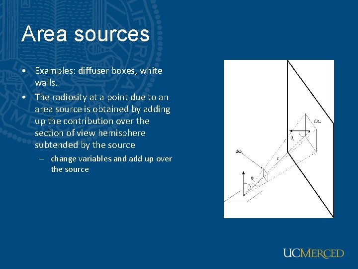
Area sources • Examples: diffuser boxes, white walls. • The radiosity at a point due to an area source is obtained by adding up the contribution over the section of view hemisphere subtended by the source – change variables and add up over the source

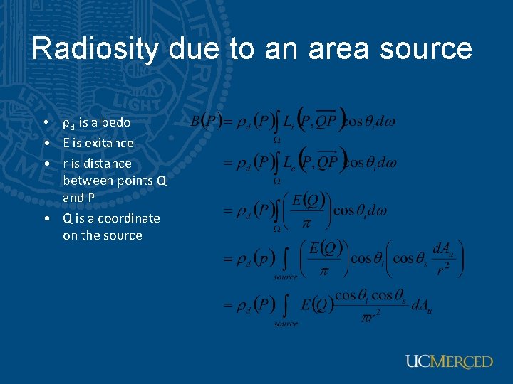
Radiosity due to an area source • ρd is albedo • E is exitance • r is distance between points Q and P • Q is a coordinate on the source

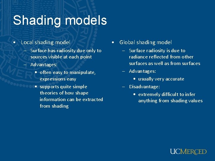
Shading models • Local shading model – Surface has radiosity due only to sources visible at each point – Advantages: • often easy to manipulate, expressions easy • supports quite simple theories of how shape information can be extracted from shading • Global shading model – Surface radiosity is due to radiance reflected from other surfaces as well as from surfaces – Advantages: • usually very accurate – Disadvantage: • extremely difficult to infer anything from shading values

Local shading models • For point sources at infinity: • For point sources not at infinity

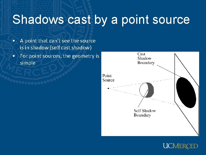
Shadows cast by a point source • A point that can’t see the source is in shadow (self cast shadow) • For point sources, the geometry is simple

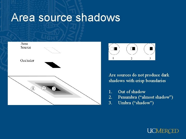
Area source shadows Are sources do not produce dark shadows with crisp boundaries 1. 2. 3. Out of shadow Penumbra (“almost shadow”) Umbra (“shadow”)

Photometric stereo • Assume: – A local shading model – A set of point sources that are infinitely distant – A set of pictures of an object, obtained in exactly the same camera/object configuration but using different sources – A Lambertian object (or the specular component has been identified and removed)

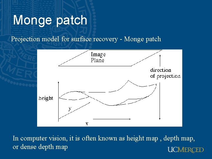
Monge patch Projection model for surface recovery - Monge patch In computer vision, it is often known as height map , depth map, or dense depth map

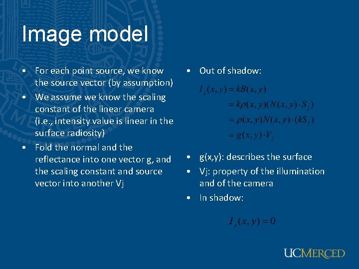
Image model • For each point source, we know the source vector (by assumption) • We assume we know the scaling constant of the linear camera (i. e. , intensity value is linear in the surface radiosity) • Fold the normal and the reflectance into one vector g, and the scaling constant and source vector into another Vj • Out of shadow: • g(x, y): describes the surface • Vj: property of the illumination and of the camera • In shadow:

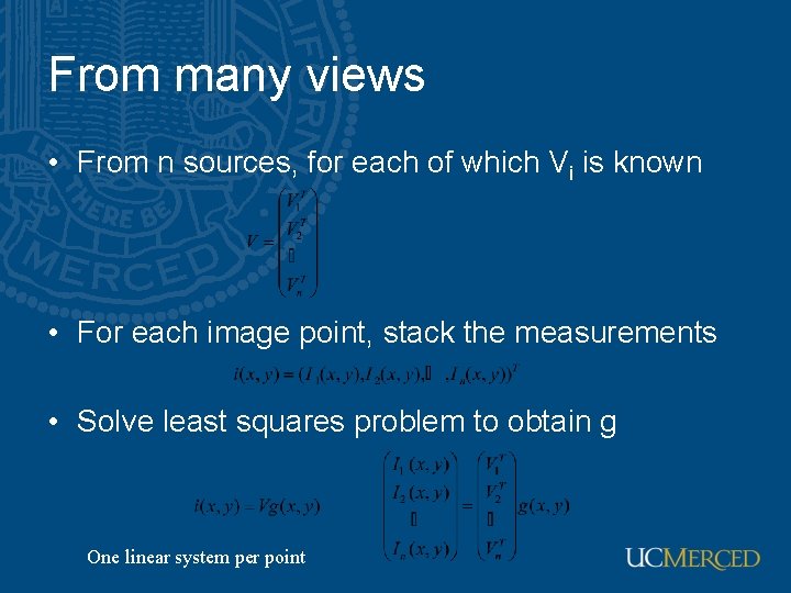
From many views • From n sources, for each of which Vi is known • For each image point, stack the measurements • Solve least squares problem to obtain g One linear system per point

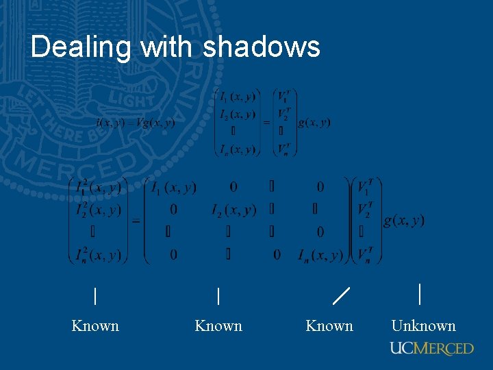
Dealing with shadows Known Unknown

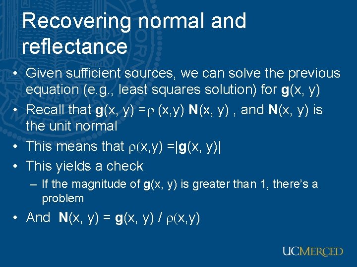
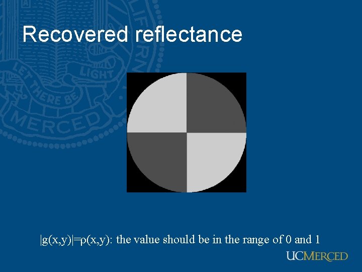
Recovering normal and reflectance • Given sufficient sources, we can solve the previous equation (e. g. , least squares solution) for g(x, y) • Recall that g(x, y) =r (x, y) N(x, y) , and N(x, y) is the unit normal • This means that r(x, y) =|g(x, y)| • This yields a check – If the magnitude of g(x, y) is greater than 1, there’s a problem • And N(x, y) = g(x, y) / r(x, y)

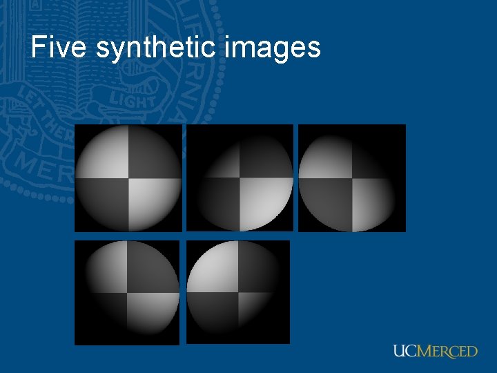
Five synthetic images

Recovered reflectance |g(x, y)|=ρ(x, y): the value should be in the range of 0 and 1

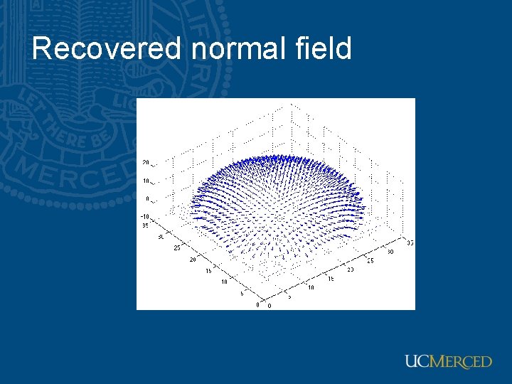
Recovered normal field

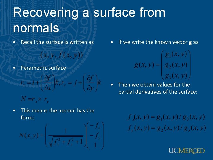
Recovering a surface from normals • Recall the surface is written as • If we write the known vector g as • Parametric surface • Then we obtain values for the partial derivatives of the surface: • This means the normal has the form:

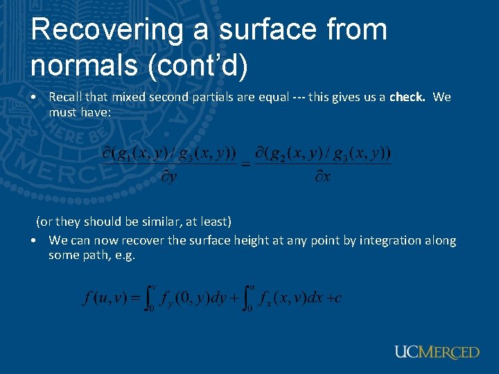
Recovering a surface from normals (cont’d) • Recall that mixed second partials are equal --- this gives us a check. We must have: (or they should be similar, at least) • We can now recover the surface height at any point by integration along some path, e. g.

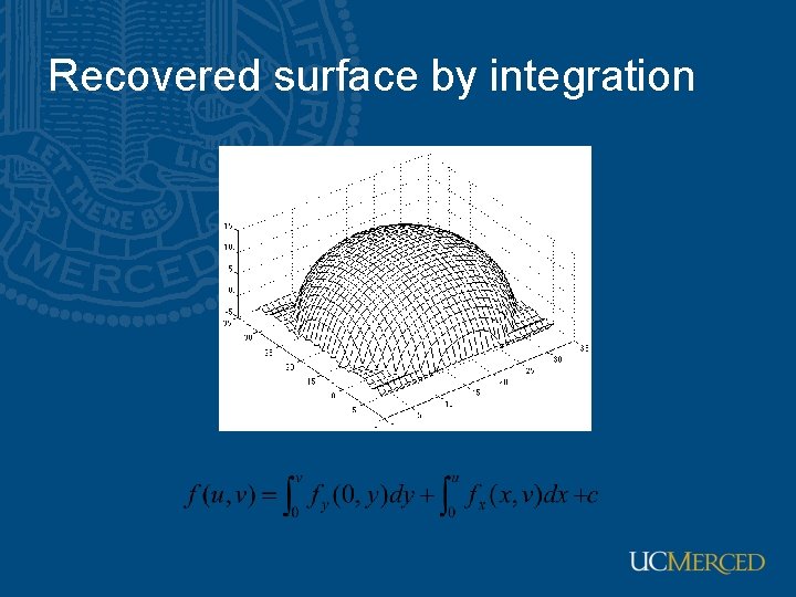
Recovered surface by integration

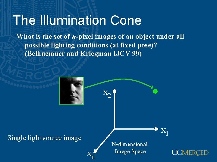
The Illumination Cone What is the set of n-pixel images of an object under all possible lighting conditions (at fixed pose)? (Belhuemuer and Kriegman IJCV 99) x 2 x 1 Single light source image xn N-dimensional Image Space

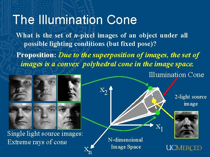
The Illumination Cone What is the set of n-pixel images of an object under all possible lighting conditions (but fixed pose)? Proposition: Due to the superposition of images, the set of images is a convex polyhedral cone in the image space. Illumination Cone x 2 Single light source images: Extreme rays of cone 2 -light source image x 1 xn N-dimensional Image Space

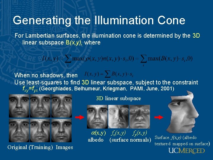
Generating the Illumination Cone For Lambertian surfaces, the illumination cone is determined by the 3 D linear subspace B(x, y), where When no shadows, then Use least-squares to find 3 D linear subspace, subject to the constraint fxy=fyx (Georghiades, Belhumeur, Kriegman, PAMI, June, 2001) 3 D linear subspace a(x, y) fx(x, y) albedo Original (Training) Images fy(x, y) (surface normals) Surface. f(x, y) (albedo textured mapped on surface)

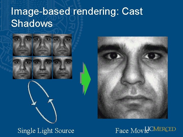
Image-based rendering: Cast Shadows Single Light Source Face Movie

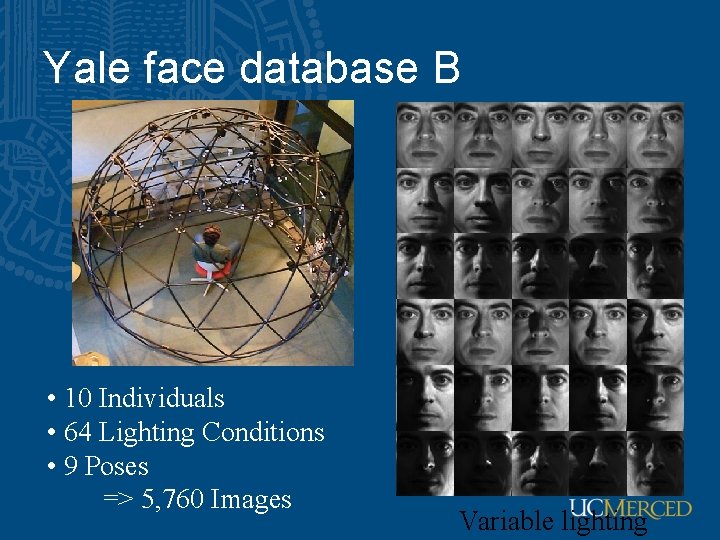
Yale face database B • 10 Individuals • 64 Lighting Conditions • 9 Poses => 5, 760 Images Variable lighting

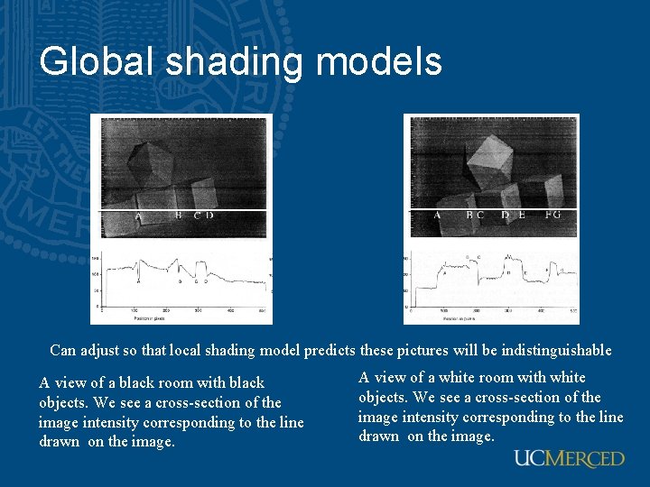
Curious experimental fact • Prepare two rooms, one with white walls and white objects, one with black walls and black objects • Illuminate the black room with bright light, the white room with dim light • People can tell which is which (due to Gilchrist) • Why? (a local shading model predicts they can’t).

Global shading models Can adjust so that local shading model predicts these pictures will be indistinguishable A view of a black room with black objects. We see a cross-section of the image intensity corresponding to the line drawn on the image. A view of a white room with white objects. We see a cross-section of the image intensity corresponding to the line drawn on the image.

What’s going on here? • Local shading model is a poor description of physical processes that give rise to images – because surfaces reflect light onto one another • This is a major nuisance; the distribution of light (in principle) depends on the configuration of every radiator; big distant ones are as important as small nearby ones (solid angle) • The effects are easy to model • It appears to be hard to extract information from these models

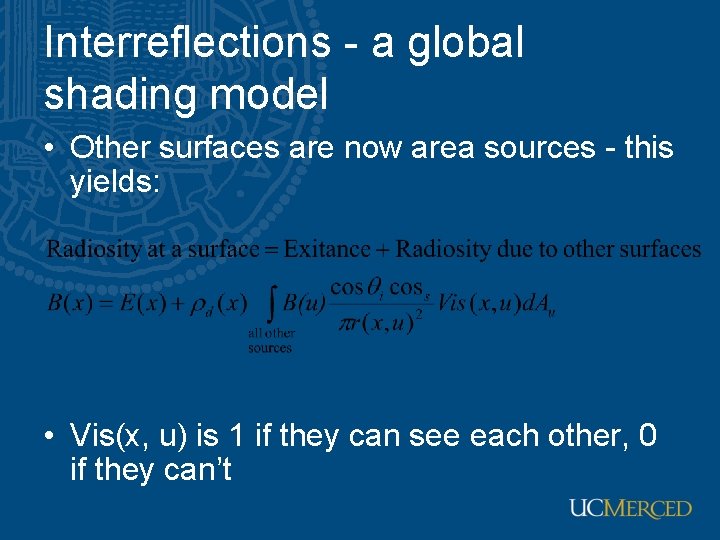
Interreflections - a global shading model • Other surfaces are now area sources - this yields: • Vis(x, u) is 1 if they can see each other, 0 if they can’t

What do we do about this? • Attempt to build approximations – Ambient illumination • Study qualitative effects – reflexes – decreased dynamic range – smoothing • Try to use other information to control errors

Ambient illumination • Two forms – Add a constant to the radiosity at every point in the scene to account for brighter shadows than predicted by point source model • Advantages: simple, easily managed (e. g. how would you change photometric stereo? ) • Disadvantages: poor approximation (compare black and white rooms – Add a term at each point that depends on the size of the clear viewing hemisphere at each point • Advantages: appears to be quite a good approximation, but jury is out • Disadvantages: difficult to work with