EECS 274 Computer Vision Geometry of Multiple Views

EECS 274 Computer Vision Geometry of Multiple Views

Geometry of Multiple Views • Epipolar geometry – Essential matrix – Fundamental matrix • Trifocal tensor • Quadrifocal tensor • Reading: FP Chapter 10, S Chapter 7

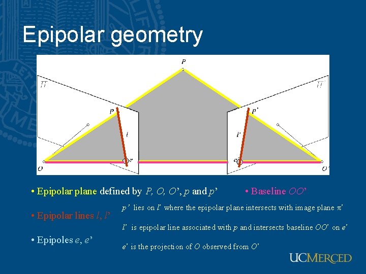
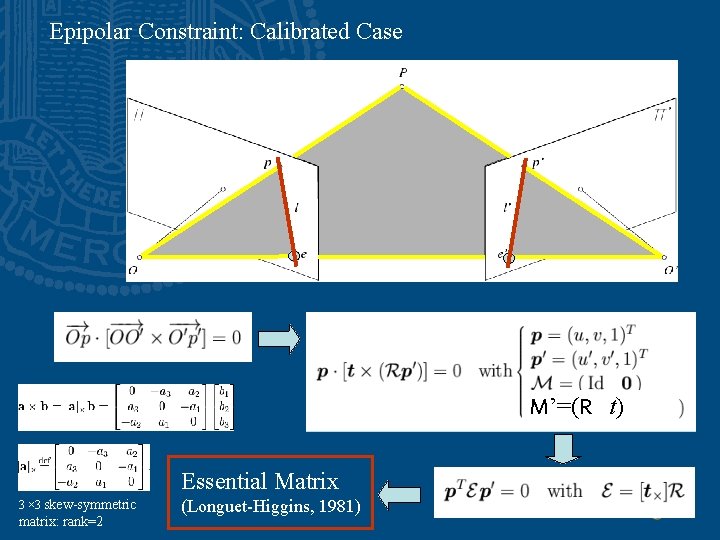
Epipolar geometry • Epipolar plane defined by P, O, O’, p and p’ • Epipolar lines l, l’ • Baseline OO’ p’ lies on l’ where the epipolar plane intersects with image plane π’ l’ is epipolar line associated with p and intersects baseline OO’ on e’ • Epipoles e, e’ e’ is the projection of O observed from O’

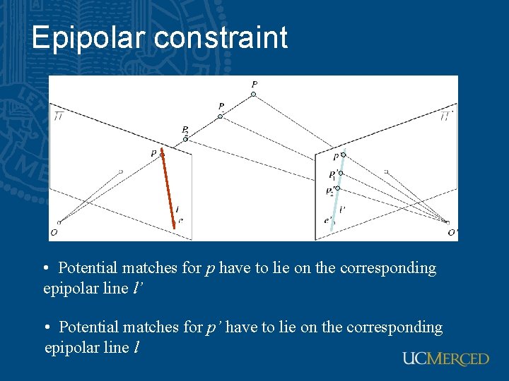
Epipolar constraint • Potential matches for p have to lie on the corresponding epipolar line l’ • Potential matches for p’ have to lie on the corresponding epipolar line l

Epipolar Constraint: Calibrated Case M’=(R t) Essential Matrix 3 × 3 skew-symmetric matrix: rank=2 (Longuet-Higgins, 1981)

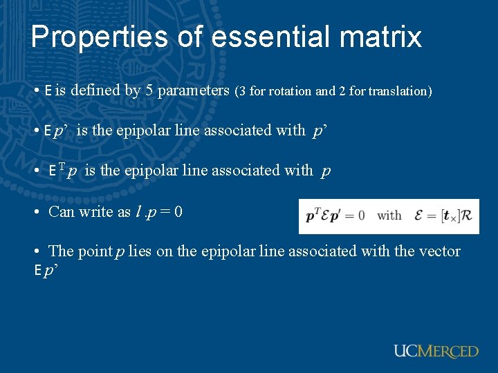
Properties of essential matrix • E is defined by 5 parameters (3 for rotation and 2 for translation) • E p’ is the epipolar line associated with p’ • E T p is the epipolar line associated with p • Can write as l. p = 0 • The point p lies on the epipolar line associated with the vector E p’

Properties of essential matrix (cont’d) • E e’=0 and ETe=0 (E e’=-RT[tx]e=0 ) • E is singular • E has two equal non-zero singular values (Huang and Faugeras, 1989)

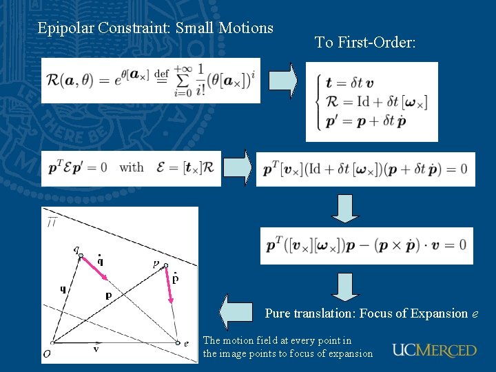
Epipolar Constraint: Small Motions To First-Order: Pure translation: Focus of Expansion e The motion field at every point in the image points to focus of expansion

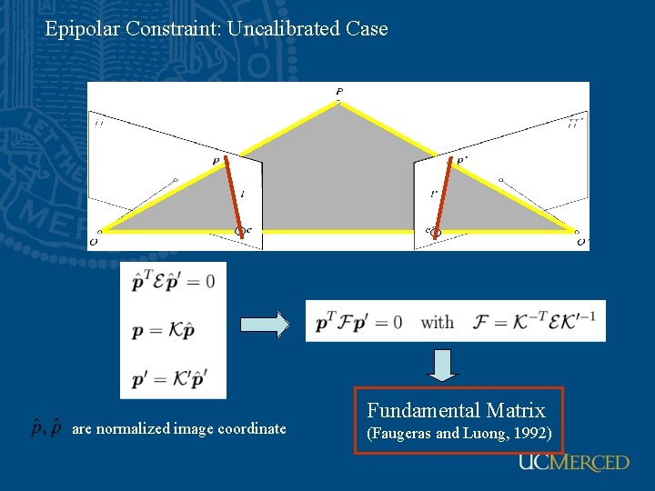
Epipolar Constraint: Uncalibrated Case are normalized image coordinate Fundamental Matrix (Faugeras and Luong, 1992)

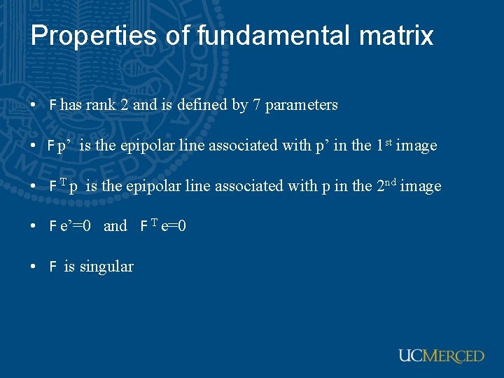
Properties of fundamental matrix • F has rank 2 and is defined by 7 parameters • F p’ is the epipolar line associated with p’ in the 1 st image • F T p is the epipolar line associated with p in the 2 nd image • F e’=0 and F T e=0 • F is singular

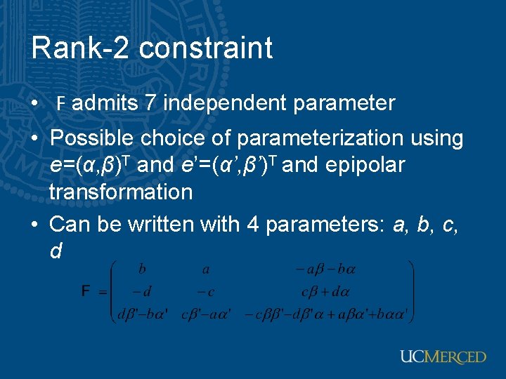
Rank-2 constraint • F admits 7 independent parameter • Possible choice of parameterization using e=(α, β)T and e’=(α’, β’)T and epipolar transformation • Can be written with 4 parameters: a, b, c, d

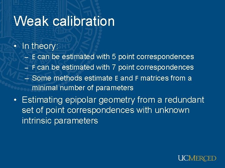
Weak calibration • In theory: – E can be estimated with 5 point correspondences – F can be estimated with 7 point correspondences – Some methods estimate E and F matrices from a minimal number of parameters • Estimating epipolar geometry from a redundant set of point correspondences with unknown intrinsic parameters

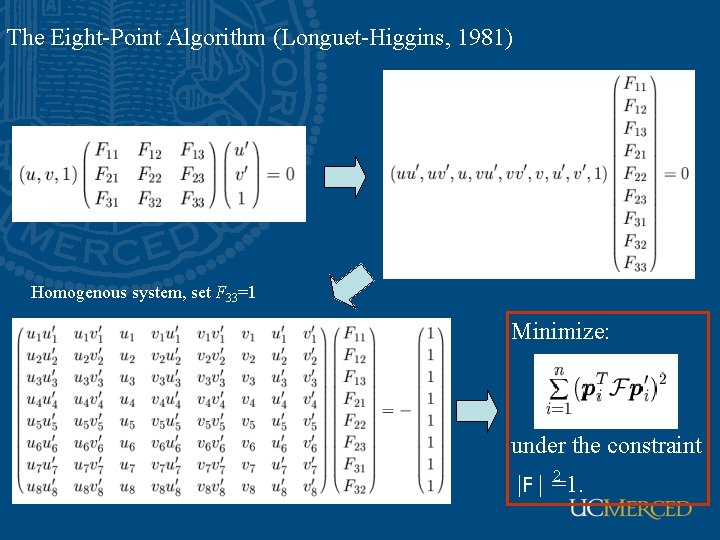
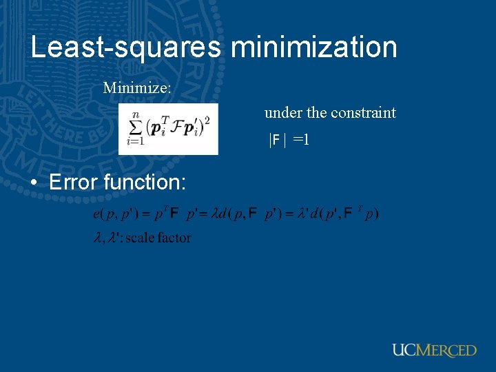
The Eight-Point Algorithm (Longuet-Higgins, 1981) Homogenous system, set F 33=1 Minimize: under the constraint 2 |F | =1.

Least-squares minimization Minimize: under the constraint |F | =1 • Error function:

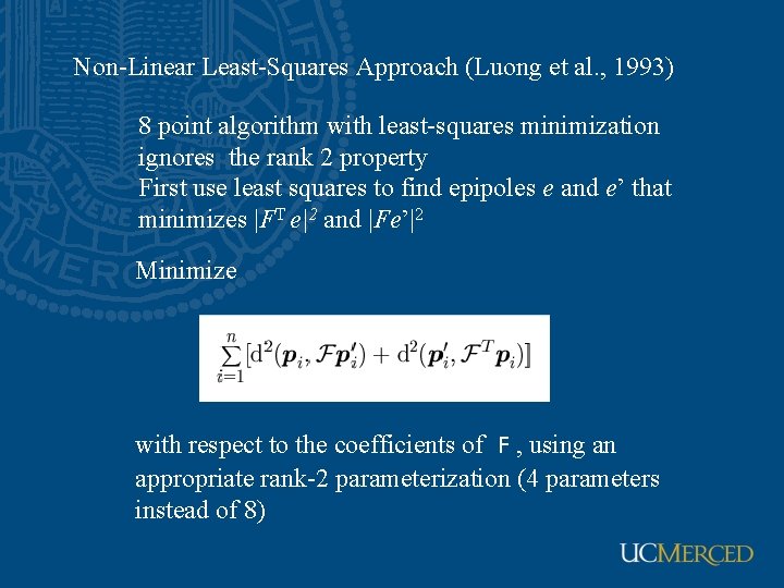
Non-Linear Least-Squares Approach (Luong et al. , 1993) 8 point algorithm with least-squares minimization ignores the rank 2 property First use least squares to find epipoles e and e’ that minimizes |FT e|2 and |Fe’|2 Minimize with respect to the coefficients of F , using an appropriate rank-2 parameterization (4 parameters instead of 8)

The Normalized Eight-Point Algorithm (Hartley, 1995) • Estimation of transformation parameters suffer form poor numerical condition problem • Center the image data at the origin, and scale it so the mean squared distance between and the data i i i the origin i points is 2 pixels: q = T p , q’ = T’ p’ • Use thei eight-point algorithm to compute F from the i points q and q’ • Enforce the rank-2 constraint T • Output T F T’

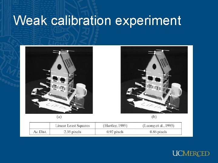
Weak calibration experiment

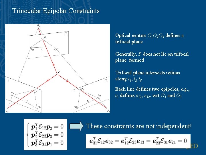
Trinocular Epipolar Constraints Optical centers O 1 O 2 O 3 defines a trifocal plane Generally, P does not lie on trifocal plane formed Trifocal plane intersects retinas along t 1, t 2, t 3 Each line defines two epipoles, e. g. , t 2 defines e 12, e 32, wrt O 1 and O 3 These constraints are not independent!

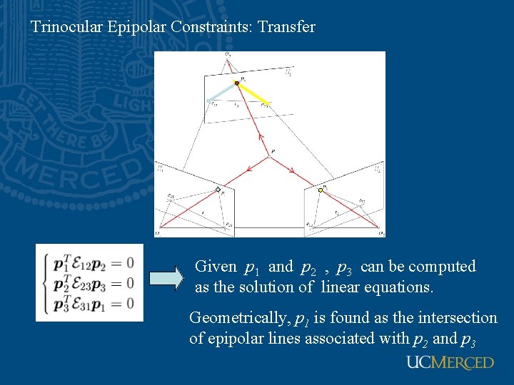
Trinocular Epipolar Constraints: Transfer Given p 1 and p 2 , p 3 can be computed as the solution of linear equations. Geometrically, p 1 is found as the intersection of epipolar lines associated with p 2 and p 3

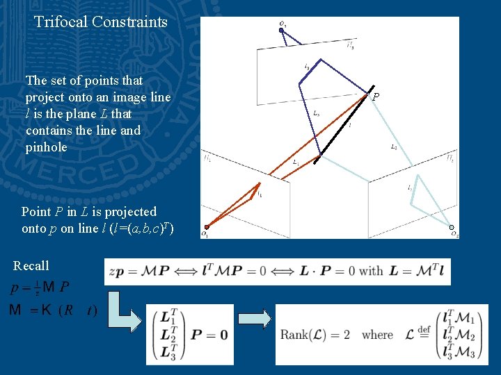
Trifocal Constraints The set of points that project onto an image line l is the plane L that contains the line and pinhole Point P in L is projected onto p on line l (l=(a, b, c)T) Recall P

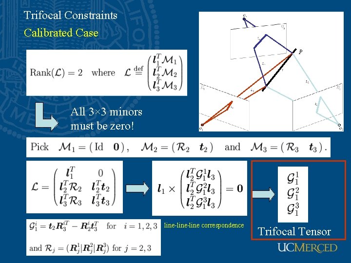
Trifocal Constraints Calibrated Case P All 3× 3 minors must be zero! line-line correspondence Trifocal Tensor

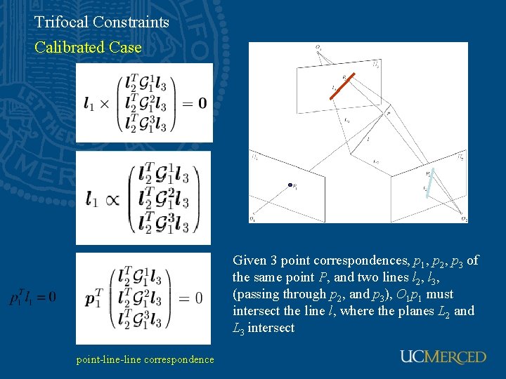
Trifocal Constraints Calibrated Case Given 3 point correspondences, p 1, p 2, p 3 of the same point P, and two lines l 2, l 3, (passing through p 2, and p 3), O 1 p 1 must intersect the line l, where the planes L 2 and L 3 intersect point-line correspondence

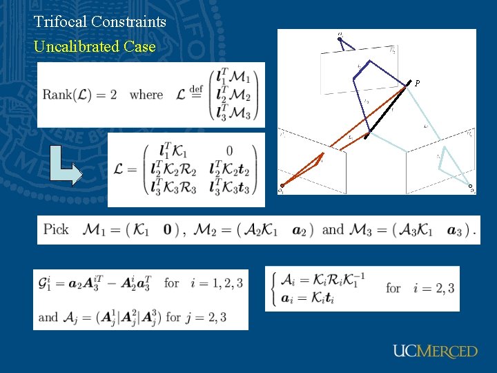
Trifocal Constraints Uncalibrated Case P

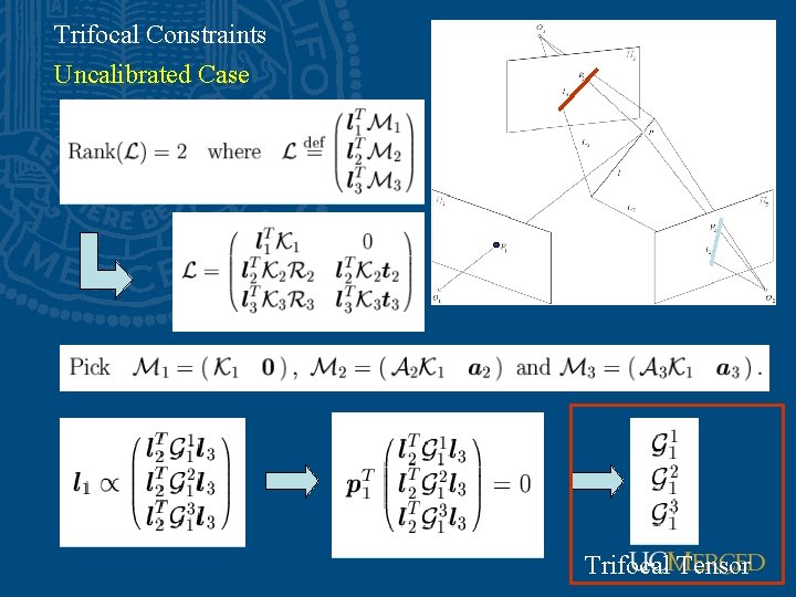
Trifocal Constraints Uncalibrated Case Trifocal Tensor

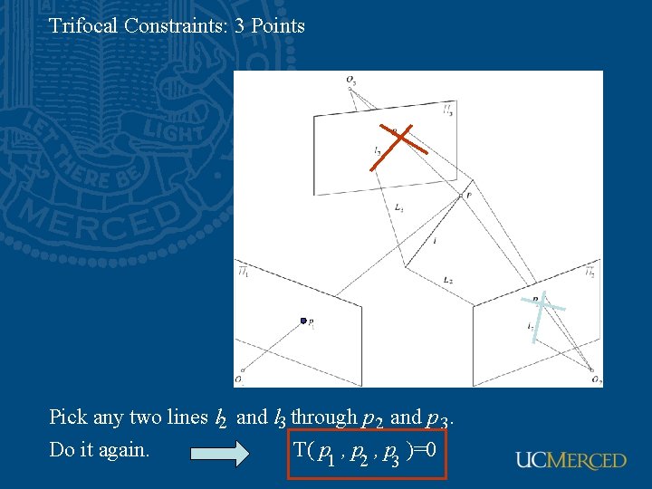
Trifocal Constraints: 3 Points Pick any two lines l 2 and l 3 through p 2 and p 3. Do it again. T( p 1 , p 2 , p )=0 3

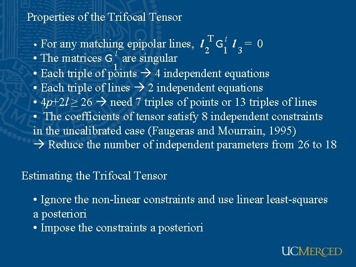
Properties of the Trifocal Tensor T i • For any matching epipolar lines, l 2 G 1 l 3 = 0 • The matrices G i are singular 1 • Each triple of points 4 independent equations • Each triple of lines 2 independent equations • 4 p+2 l ≥ 26 need 7 triples of points or 13 triples of lines • The coefficients of tensor satisfy 8 independent constraints in the uncalibrated case (Faugeras and Mourrain, 1995) Reduce the number of independent parameters from 26 to 18 Estimating the Trifocal Tensor • Ignore the non-linear constraints and use linear least-squares a posteriori • Impose the constraints a posteriori

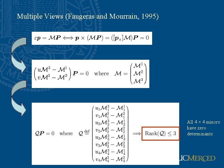
Multiple Views (Faugeras and Mourrain, 1995) All 4 × 4 minors have zero determinants

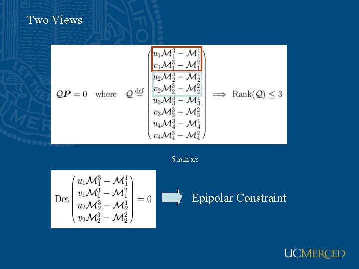
Two Views 6 minors Epipolar Constraint

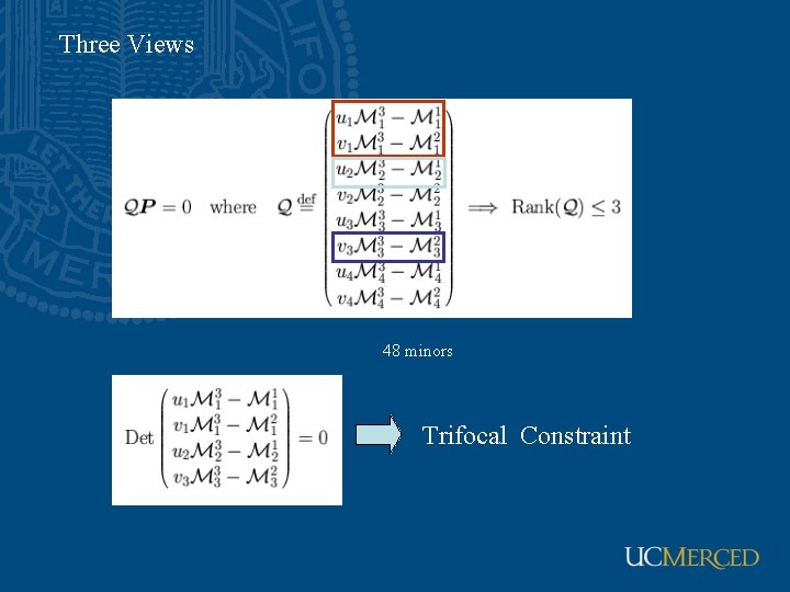
Three Views 48 minors Trifocal Constraint

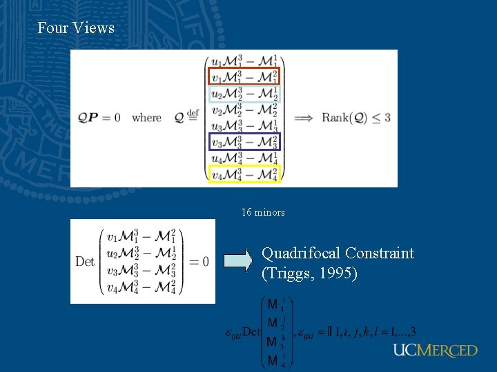
Four Views 16 minors Quadrifocal Constraint (Triggs, 1995)

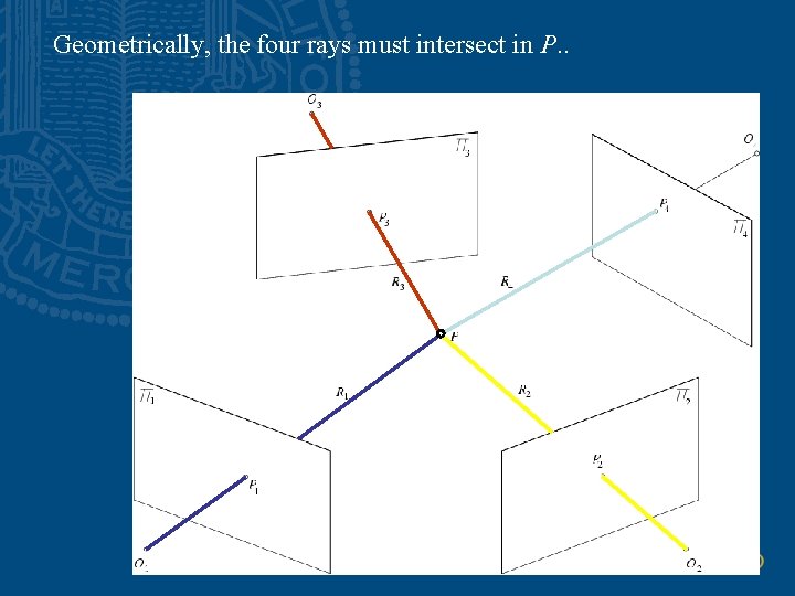
Geometrically, the four rays must intersect in P. .

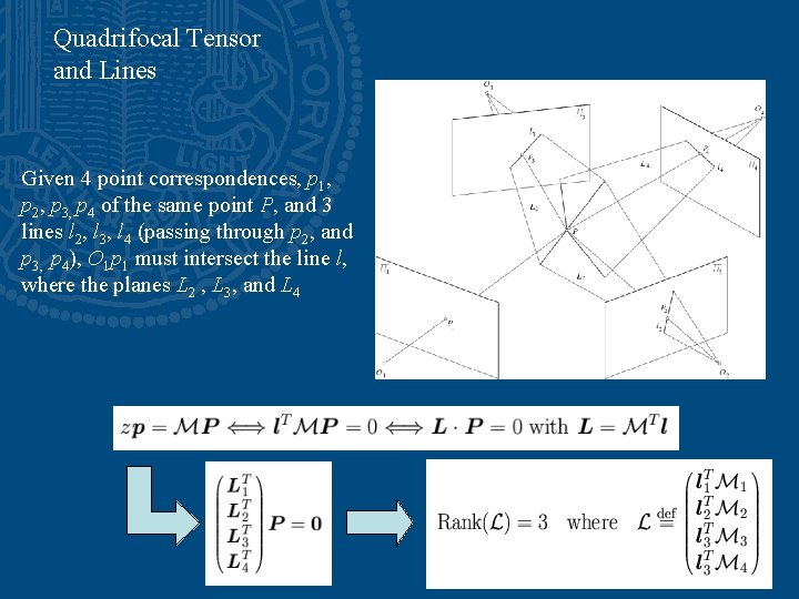
Quadrifocal Tensor and Lines Given 4 point correspondences, p 1, p 2, p 3, p 4 of the same point P, and 3 lines l 2, l 3, l 4 (passing through p 2, and p 3, p 4), O 1 p 1 must intersect the line l, where the planes L 2 , L 3, and L 4

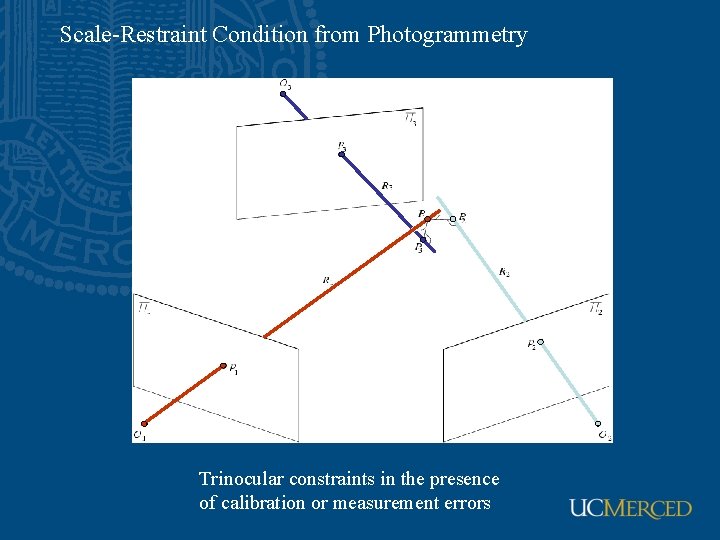
Scale-Restraint Condition from Photogrammetry Trinocular constraints in the presence of calibration or measurement errors