Deep Learning and Its Application to Signal and

Deep Learning and Its Application to Signal and Image Processing and Analysis CLASS III - SPRING 2018 TAMMY RIKLIN RAVIV, ELECTRICAL AND COMPUTER ENGINEERING

Two ML talks this week Today, 13: 00 Spectral methods for unsupervised ensemble methods – Ariel Jaffe, Weizmann Institute Wednesday, 12: 00 On the relationship between the structure in the data and what deep learning can learn. Dr. Raja Giryes, EE, Tel-Aviv University

This class Numerical computation issues Regularization Capacity, overfitting and underfitting …. And if time let CNN

Numerical computation Rounding Underflow Overflow Poor conditioning

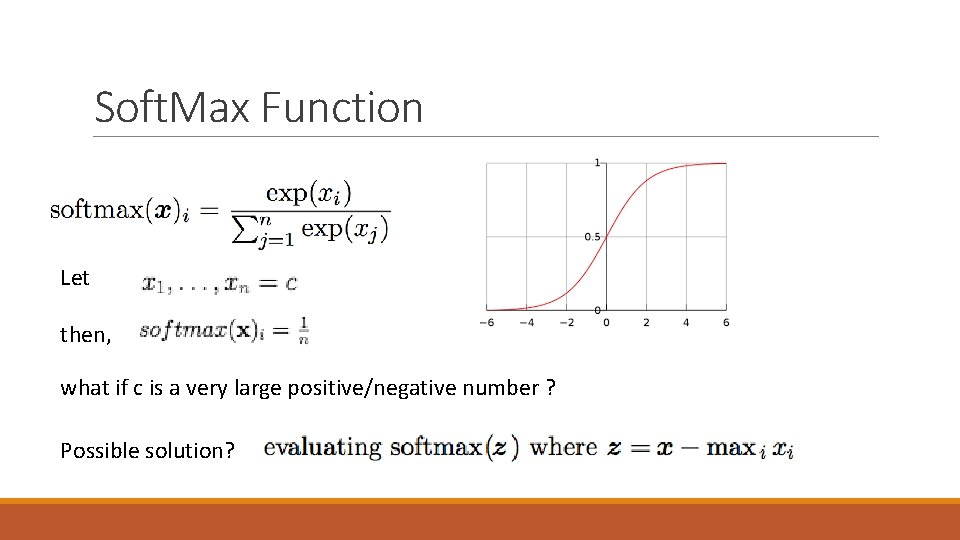
Soft. Max Function Let then, what if c is a very large positive/negative number ? Possible solution?

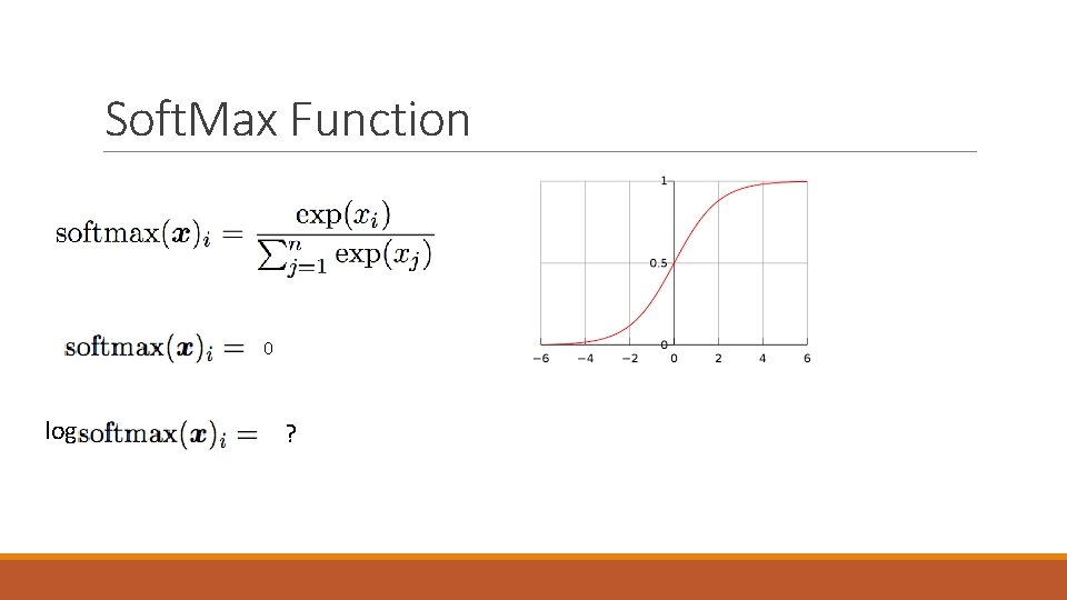
Soft. Max Function 0 log ?

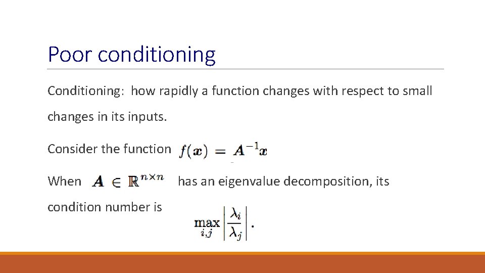
Poor conditioning Conditioning: how rapidly a function changes with respect to small changes in its inputs. Consider the function When condition number is has an eigenvalue decomposition, its

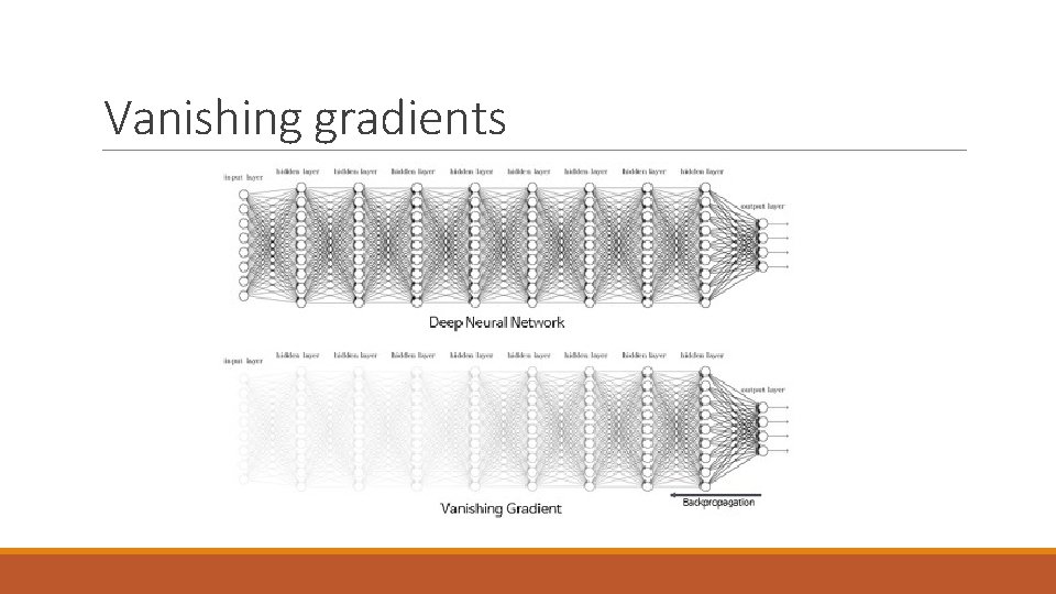
Vanishing gradients

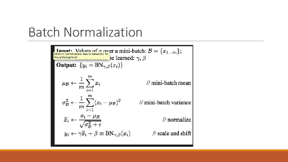
Batch Normalization

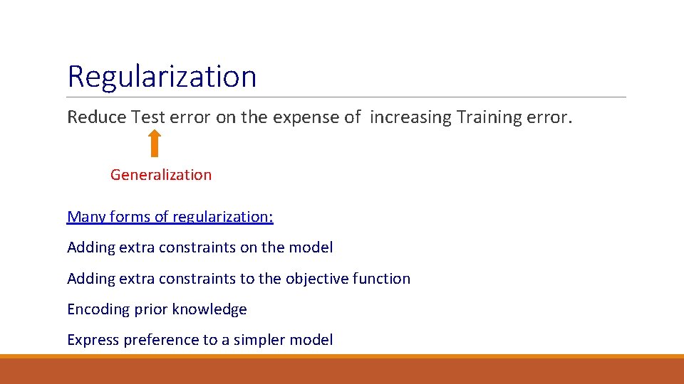
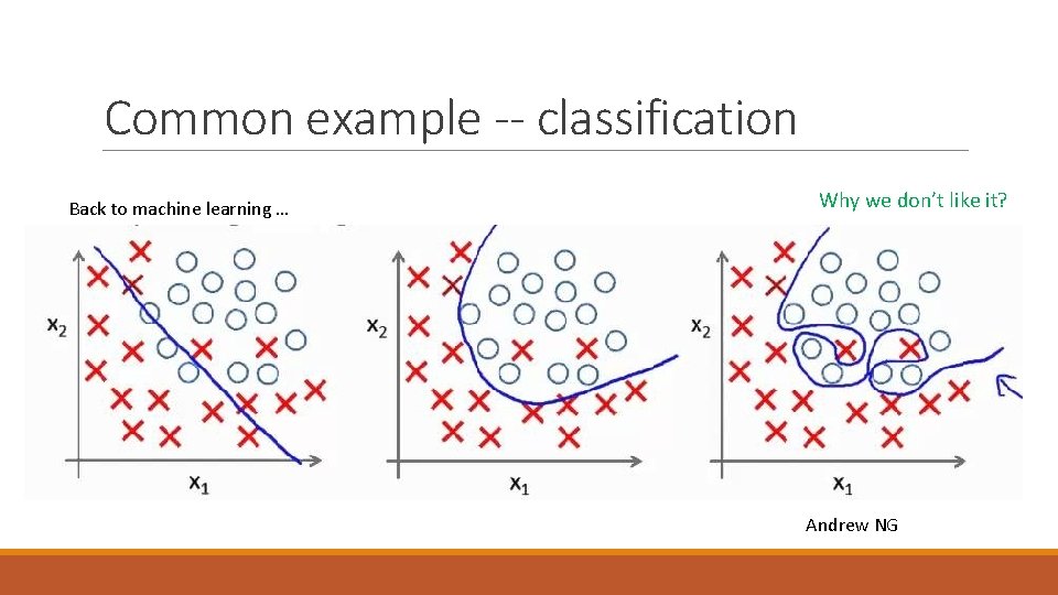
Regularization Reduce Test error on the expense of increasing Training error. Generalization Many forms of regularization: Adding extra constraints on the model Adding extra constraints to the objective function Encoding prior knowledge Express preference to a simpler model

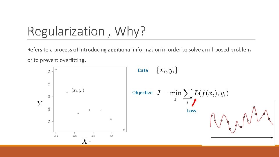
Regularization , Why? Refers to a process of introducing additional information in order to solve an ill-posed problem or to prevent overfitting. Data Objective Loss

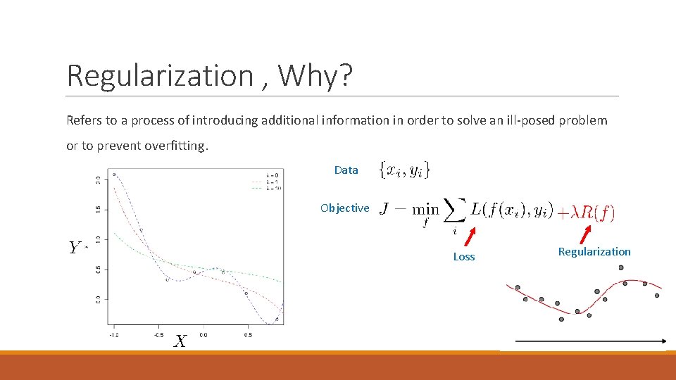
Regularization , Why? Refers to a process of introducing additional information in order to solve an ill-posed problem or to prevent overfitting. Data Objective Loss Regularization

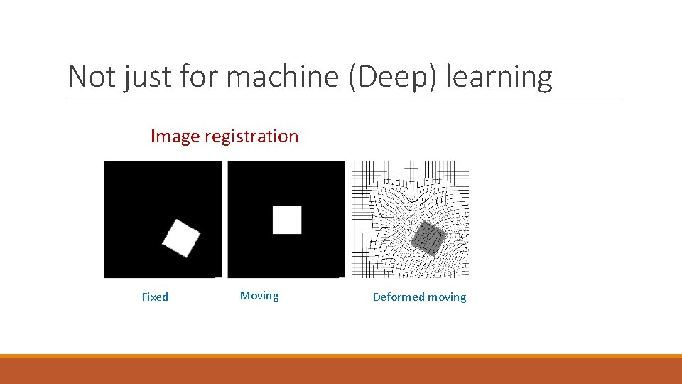
Not just for machine (Deep) learning Image registration Fixed Moving Deformed moving

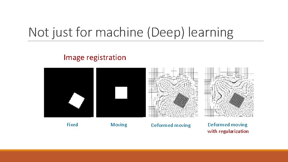
Not just for machine (Deep) learning Image registration Fixed Moving Deformed moving with regularization

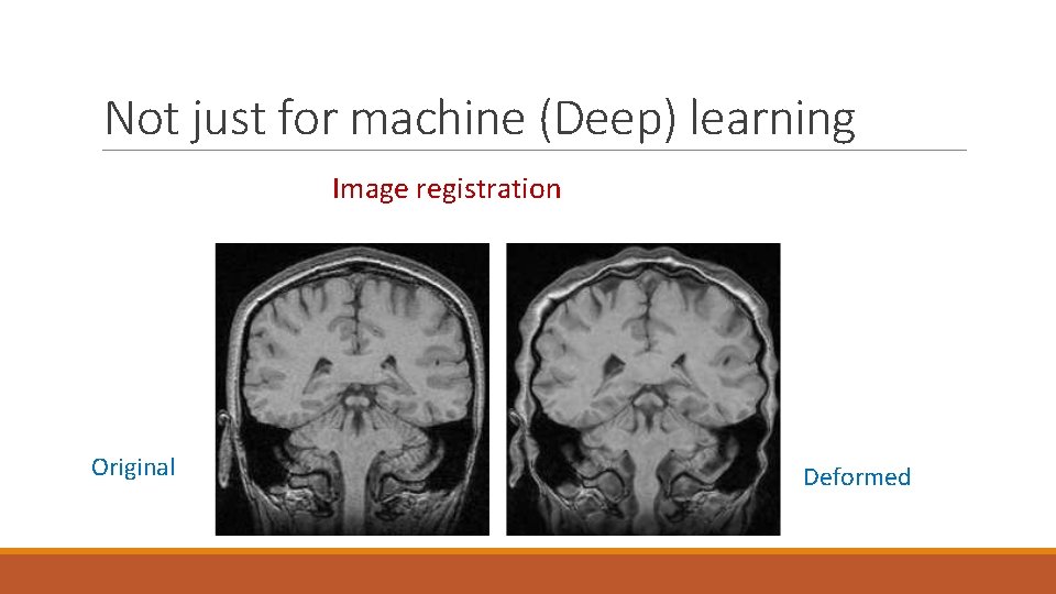
Not just for machine (Deep) learning Image registration Original Deformed

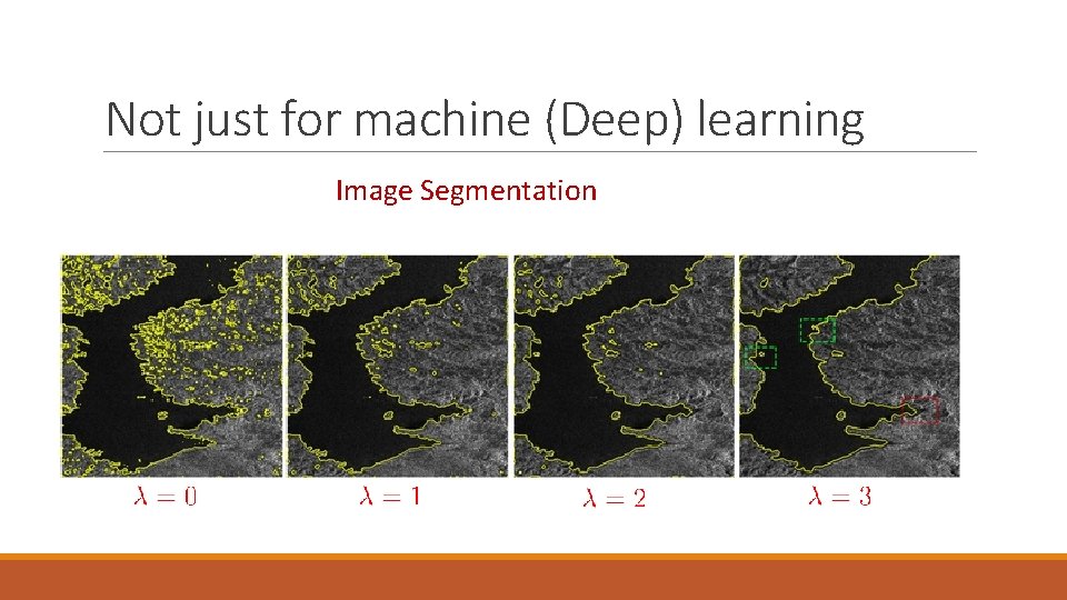
Not just for machine (Deep) learning Image Segmentation

Common example -- classification Back to machine learning … Why we don’t like it? Andrew NG

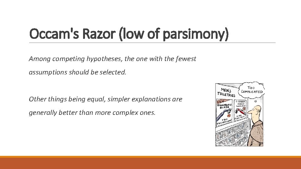
Occam's Razor (low of parsimony) Among competing hypotheses, the one with the fewest assumptions should be selected. Other things being equal, simpler explanations are generally better than more complex ones.

Common example -- classification Back to machine learning … Why we don’t like it? Andrew NG

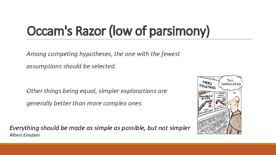
Occam's Razor (low of parsimony) Among competing hypotheses, the one with the fewest assumptions should be selected. Other things being equal, simpler explanations are generally better than more complex ones. Everything should be made as simple as possible, but not simpler Albert Einstein

Capacity, overfitting and underfitting Main challenge of machine learning algorithms – perform well on new, previously unseen inputs. Assumptions (i. i. d. ) : The train dataset and the test dataset are independent of each other and each dataset is identically distributed, drawn from the same probability distribution as each other. Observation: the expected training error of a randomly selected model should be equal to the expected test error of that model. Yet, since we set the parameters based on the training and then use the test – the test error is higher.

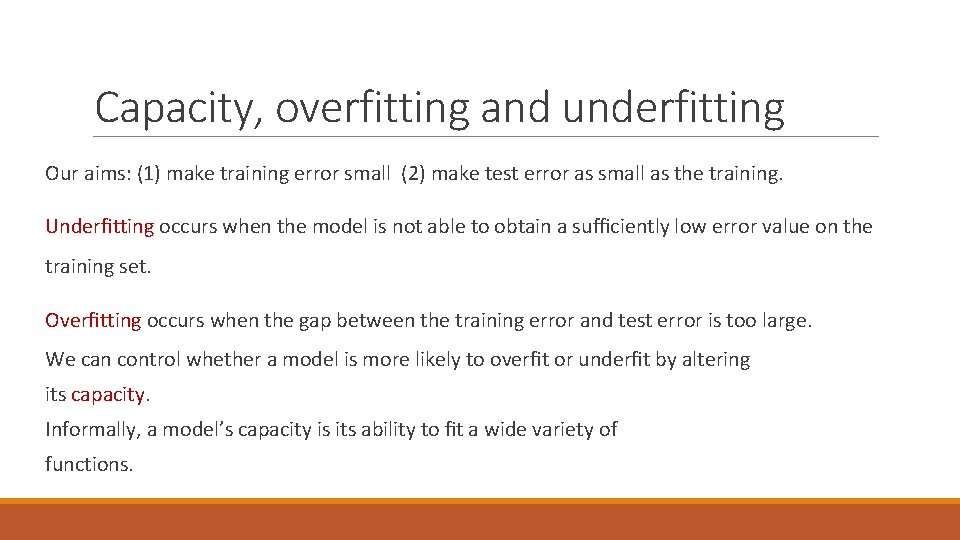
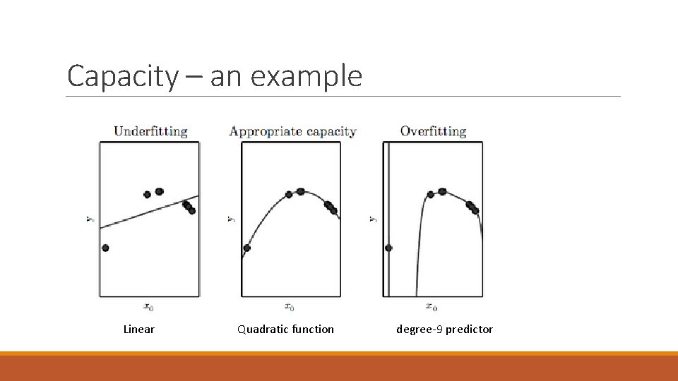
Capacity, overfitting and underfitting Our aims: (1) make training error small (2) make test error as small as the training. Underfitting occurs when the model is not able to obtain a sufficiently low error value on the training set. Overfitting occurs when the gap between the training error and test error is too large. We can control whether a model is more likely to overfit or underfit by altering its capacity. Informally, a model’s capacity is its ability to fit a wide variety of functions.

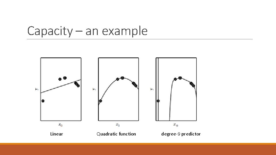
Capacity – an example Linear Quadratic function degree-9 predictor

Capacity – an example Linear Quadratic function degree-9 predictor

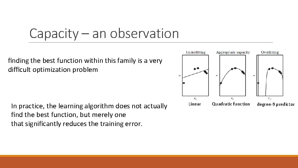
Capacity – an observation finding the best function within this family is a very difficult optimization problem In practice, the learning algorithm does not actually find the best function, but merely one that significantly reduces the training error. Linear Quadratic function degree-9 predictor

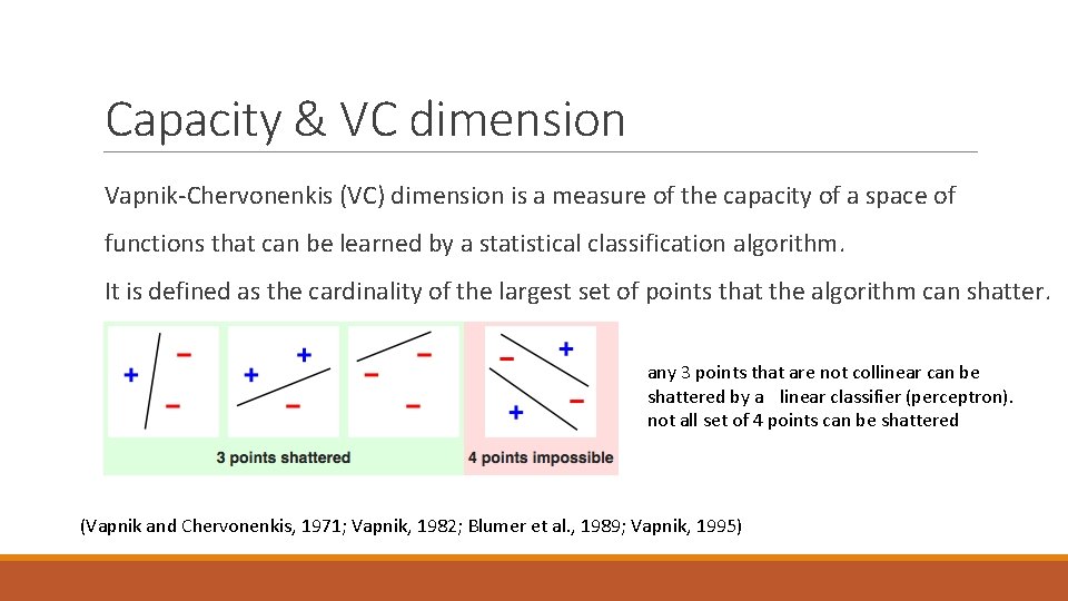
Capacity & VC dimension Vapnik-Chervonenkis (VC) dimension is a measure of the capacity of a space of functions that can be learned by a statistical classification algorithm. It is defined as the cardinality of the largest set of points that the algorithm can shatter. (Vapnik and Chervonenkis, 1971; Vapnik, 1982; Blumer et al. , 1989; Vapnik, 1995)

Capacity & VC dimension Vapnik-Chervonenkis (VC) dimension is a measure of the capacity of a space of functions that can be learned by a statistical classification algorithm. It is defined as the cardinality of the largest set of points that the algorithm can shatter. any 3 points that are not collinear can be shattered by a linear classifier (perceptron). not all set of 4 points can be shattered (Vapnik and Chervonenkis, 1971; Vapnik, 1982; Blumer et al. , 1989; Vapnik, 1995)

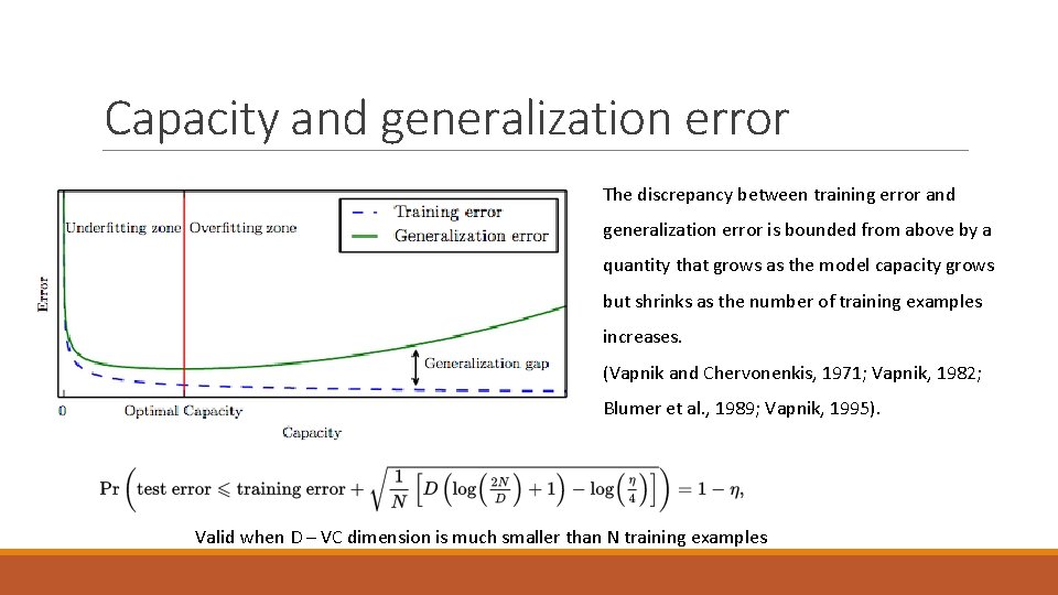
Capacity and generalization error The discrepancy between training error and generalization error is bounded from above by a quantity that grows as the model capacity grows but shrinks as the number of training examples increases. (Vapnik and Chervonenkis, 1971; Vapnik, 1982; Blumer et al. , 1989; Vapnik, 1995). Valid when D – VC dimension is much smaller than N training examples

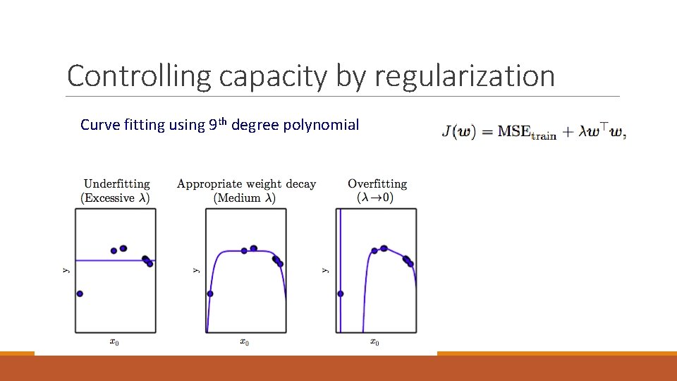
Controlling capacity by regularization Curve fitting using 9 th degree polynomial

Generalization – another philosophical note Can any Machine Learning algorithm generalize well from a finite training set of examples? To logically infer a rule describing every member of a set, one must have information about every member of that set.

Generalization – a philosophical note Can any Machine Learning algorithm generalize well from a finite training set of examples? Machine learning promises to find rules that are probably correct about most members of the set they concern.

No free lunch theorem Averaged over all possible data generating distributions, every classification algorithm has the same error rate when classifying previously unobserved points.

No free lunch theorem Averaged over all possible data generating distributions, every classification algorithm has the same error rate when classifying previously unobserved points. This means that the goal of machine learning research is not to seek a universal learning algorithm or the absolute best learning algorithm. Instead, our goal is to understand what kinds of distributions are relevant to the “real world” that an AI agent experiences, and what kinds of machine learning algorithms perform well on data drawn from the kinds of data generating distributions we care about.

Preference and Regularization The no free lunch theorem implies that we must design our machine learning algorithms to perform well on a specific task. We do so by building a set of preferences into the learning algorithm. When these preferences are aligned with the learning problems we ask the algorithm to solve, it performs better. Specifically, we can give a learning algorithm a preference for one solution in its hypothesis space to another. This means that both functions are eligible, but one is preferred. The unpreferred solution will be chosen only if it fits the training data significantly better than the preferred solution.

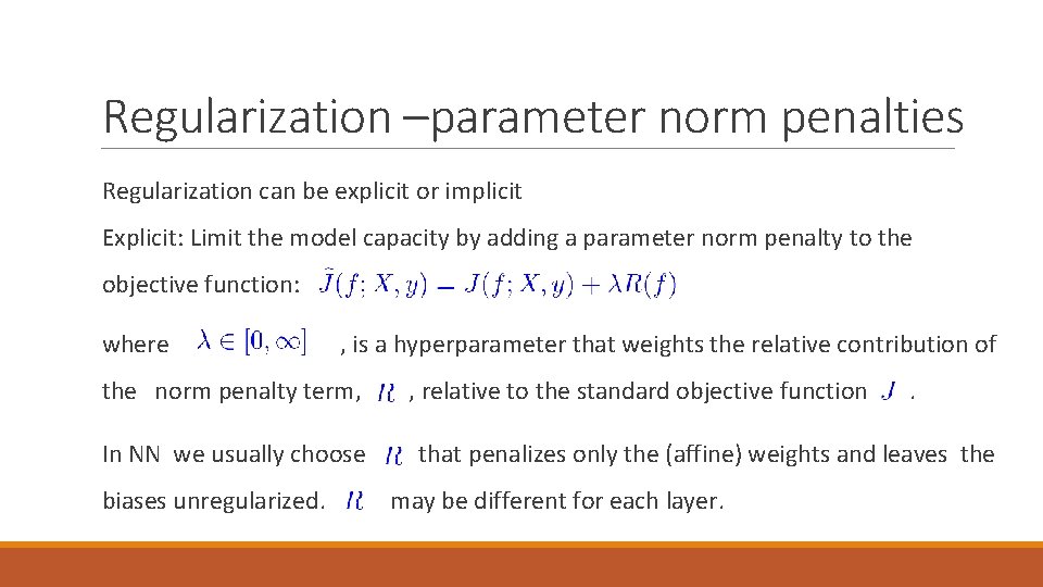
Regularization –parameter norm penalties Regularization can be explicit or implicit Explicit: Limit the model capacity by adding a parameter norm penalty to the objective function: where , is a hyperparameter that weights the relative contribution of the norm penalty term, In NN we usually choose biases unregularized. , relative to the standard objective function . that penalizes only the (affine) weights and leaves the may be different for each layer.

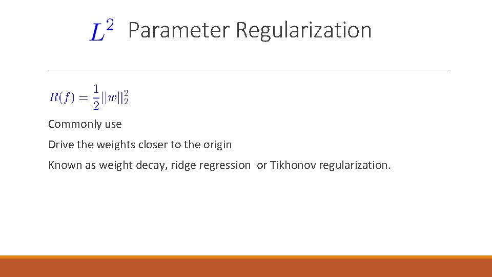
Parameter Regularization Commonly use Drive the weights closer to the origin Known as weight decay, ridge regression or Tikhonov regularization.

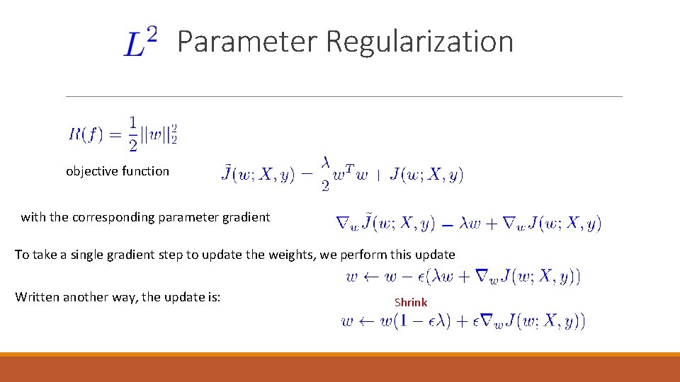
Parameter Regularization objective function with the corresponding parameter gradient To take a single gradient step to update the weights, we perform this update Written another way, the update is: Shrink

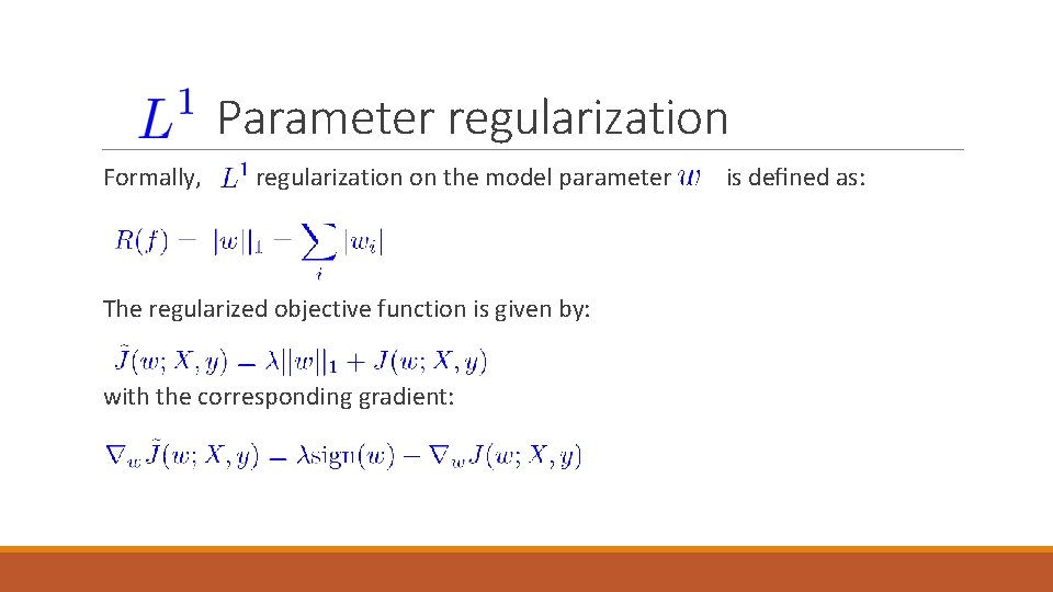
Parameter regularization Formally, regularization on the model parameter The regularized objective function is given by: with the corresponding gradient: is defined as:

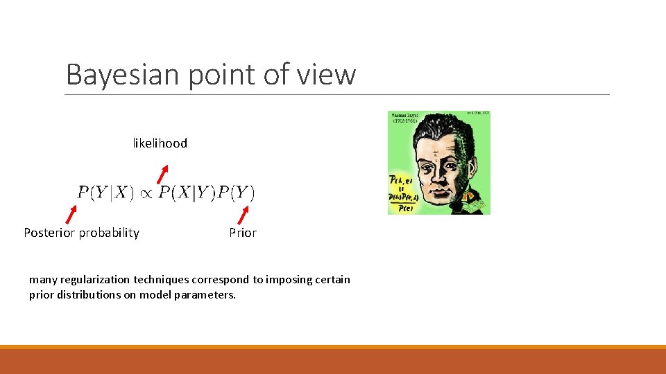
Bayesian point of view likelihood Prior Posterior probability many regularization techniques correspond to imposing certain prior distributions on model parameters.

Bayesian point of view likelihood Posterior probability Prior many regularization techniques correspond to imposing certain prior distributions on model parameters.

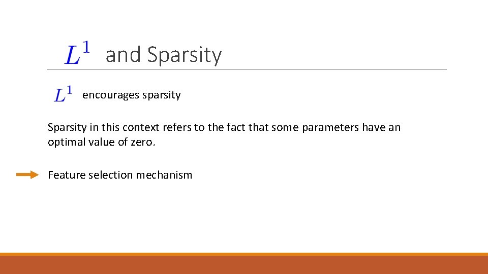
and Sparsity encourages sparsity Sparsity in this context refers to the fact that some parameters have an optimal value of zero. Feature selection mechanism

Early stopping can be viewed as regularization in time. Intuitively, a training procedure like gradient descent will tend to learn more and more complex functions as the number of iterations increases. By regularizing on time, the complexity of the model can be controlled, improving generalization. In practice, early stopping is implemented by training on a training set and measuring accuracy on a statistically independent validation set. The model is trained until performance on the validation set no longer improves. The model is then tested on a testing set.

Bagging and Other Ensemble Methods Bagging (bootstrap aggregating) is a technique for reducing generalization error by combining several models (Breiman, 1994). The idea is to train several different models separately, then have all of the models vote on the output for test examples. Models using averaging techniques are called ensemble methods The reason that model averaging works is that different models will usually not make all the same errors on the test set. On average, the ensemble will perform at least as well as any of its members, and if the members make independent errors, the ensemble will perform significantly better than its members

Regularization for Deep Learning Overfitting, underfitting and capacity Parameter norm penalties parameter regularization Main resource: Deep learning book, chapter 7 Goodfellow and Bengio and Courville MIT Press, 2016 regularization Early stopping Bagging Some other forms (implicit) of regularization, e. g. Dropout will be discussed later.

Regularization for Deep Learning Bias is not regularized Different layers – sometimes different regularization Main resource: Deep learning book, chapter 7 Goodfellow and Bengio and Courville MIT Press, 2016

Rest of Today’s plan Convolutional Neural Networks Convolution and Pooling Different variants Main resource: Deep learning book, chapter 9 Goodfellow and Bengio and Courville MIT Press, 2016 Different Data types & dimensions Different applications How to make more efficient ? Case studies Tensor Flow 50

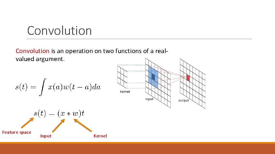
Convolution is an operation on two functions of a realvalued argument. Feature space Input Kernel

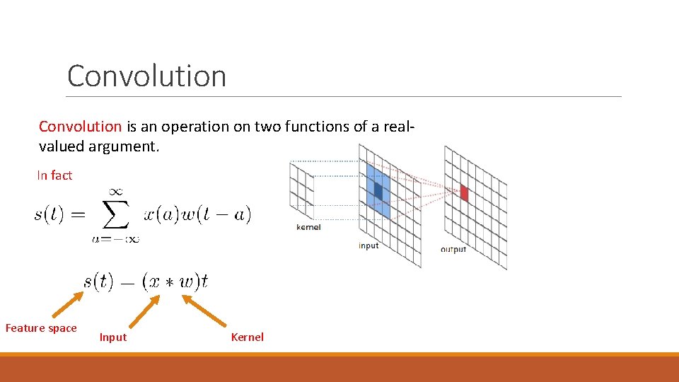
Convolution is an operation on two functions of a realvalued argument. In fact Feature space Input Kernel

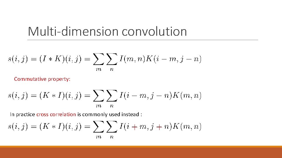
Multi-dimension convolution Commutative property: In practice cross correlation is commonly used instead :

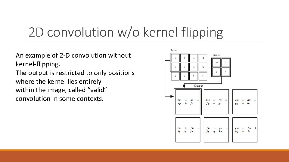
2 D convolution w/o kernel flipping An example of 2 -D convolution without kernel-flipping. The output is restricted to only positions where the kernel lies entirely within the image, called “valid” convolution in some contexts.

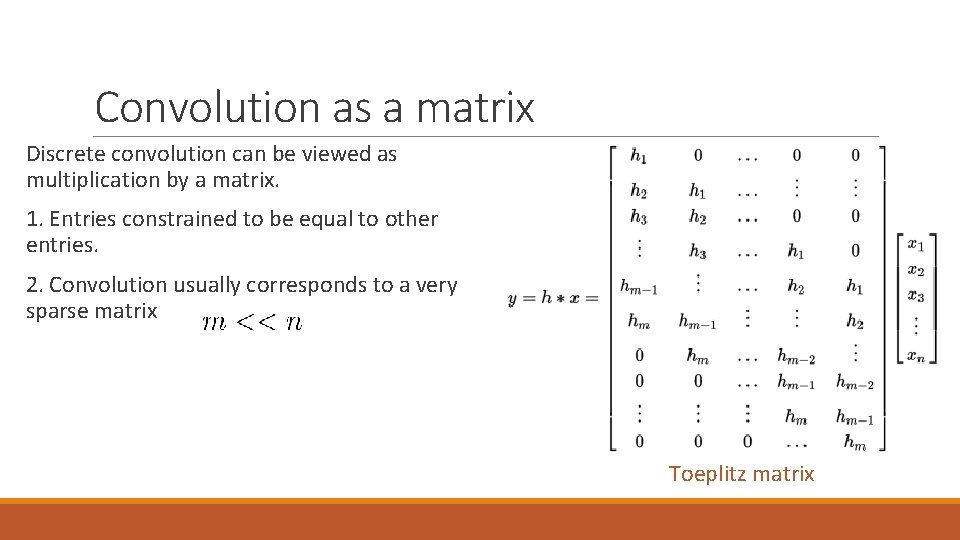
Convolution as a matrix Discrete convolution can be viewed as multiplication by a matrix. 1. Entries constrained to be equal to other entries. 2. Convolution usually corresponds to a very sparse matrix Toeplitz matrix

Convolution – three key ideas 1. Sparse interactions 2. Parameter sharing 3. Equivariant representations.

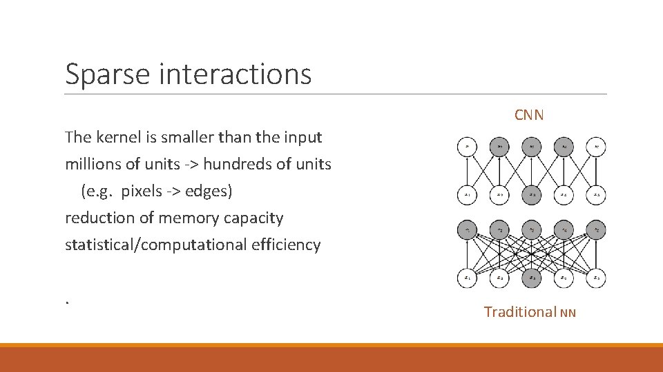
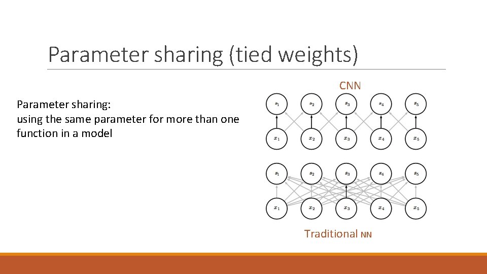
Sparse interactions CNN The kernel is smaller than the input millions of units -> hundreds of units (e. g. pixels -> edges) reduction of memory capacity statistical/computational efficiency. Traditional NN

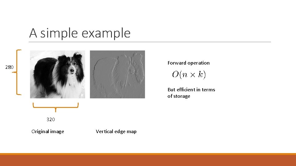
A simple example Forward operation 280 But efficient in terms of storage 320 Original image Vertical edge map

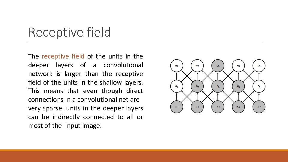
Receptive field The receptive field of the units in the deeper layers of a convolutional network is larger than the receptive field of the units in the shallow layers. This means that even though direct connections in a convolutional net are very sparse, units in the deeper layers can be indirectly connected to all or most of the input image.

Parameter sharing (tied weights) CNN Parameter sharing: using the same parameter for more than one function in a model Traditional NN

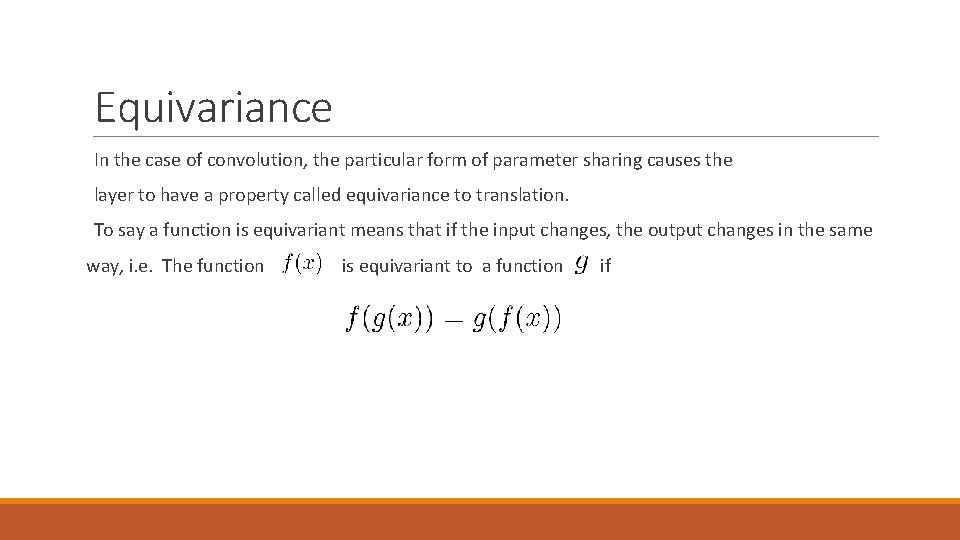
Equivariance In the case of convolution, the particular form of parameter sharing causes the layer to have a property called equivariance to translation. To say a function is equivariant means that if the input changes, the output changes in the same way, i. e. The function is equivariant to a function if

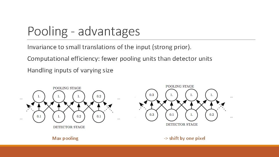
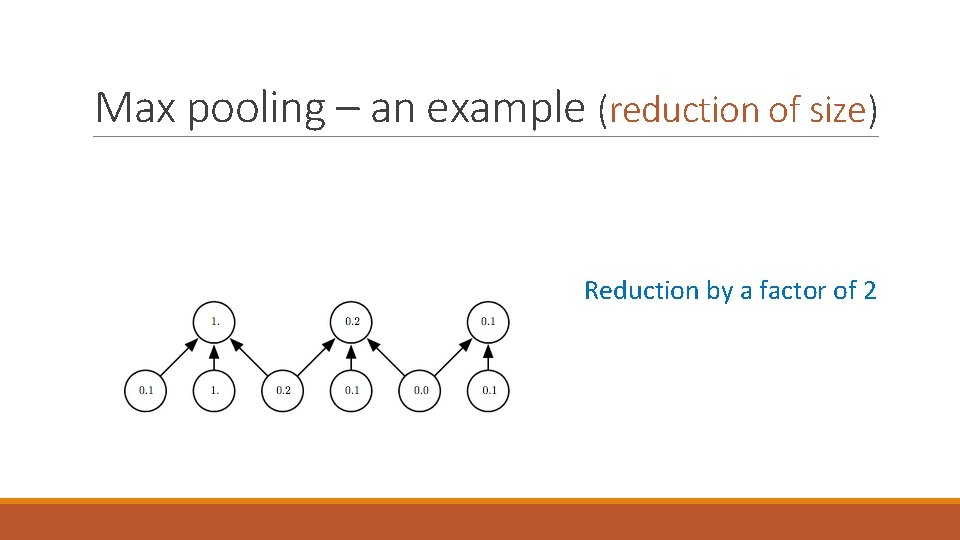
Pooling A pooling function replaces the output of the net at a certain location with a summary statistic of the nearby outputs (e. g. a rectangle neighborhood). 1. Max pooling 2. Average 3. Weighted average (e. g. based on the distance from the central voxel) 4. L 2 Norm

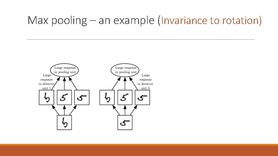
Pooling - advantages Invariance to small translations of the input (strong prior). Computational efficiency: fewer pooling units than detector units Handling inputs of varying size Max pooling -> shift by one pixel

Max pooling – an example (Invariance to rotation)

Max pooling – an example (reduction of size) Reduction by a factor of 2

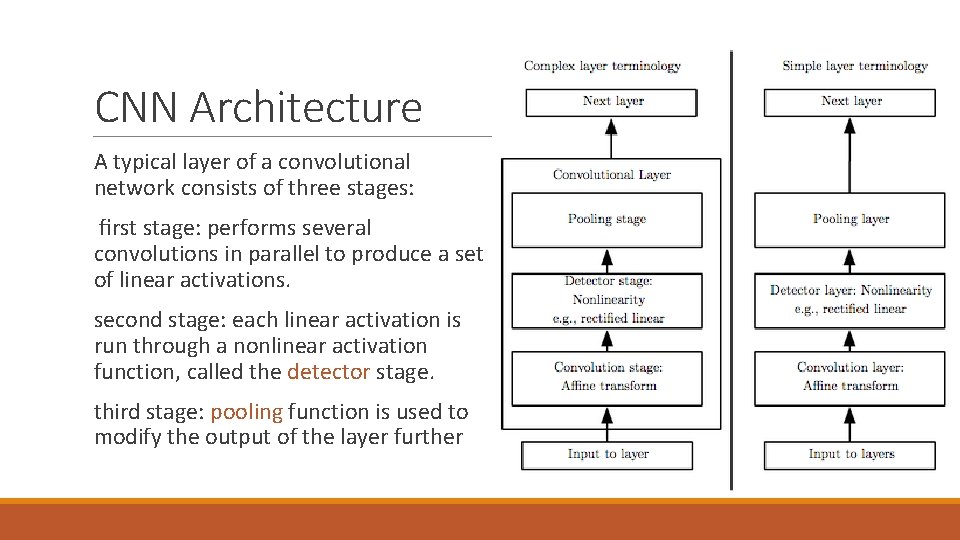
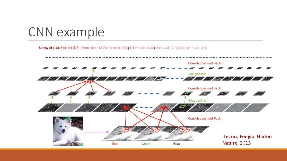
CNN Architecture A typical layer of a convolutional network consists of three stages: first stage: performs several convolutions in parallel to produce a set of linear activations. second stage: each linear activation is run through a nonlinear activation function, called the detector stage. third stage: pooling function is used to modify the output of the layer further

CNN example Le. Cun, Bengio, Hinton Nature, 2015

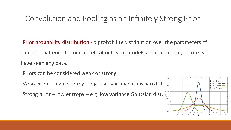
Convolution and Pooling as an Infinitely Strong Prior probability distribution - a probability distribution over the parameters of a model that encodes our beliefs about what models are reasonable, before we have seen any data. Priors can be considered weak or strong. Weak prior – high entropy – e. g. high variance Gaussian dist. Strong prior – low entropy – e. g. low variance Gaussian dist.

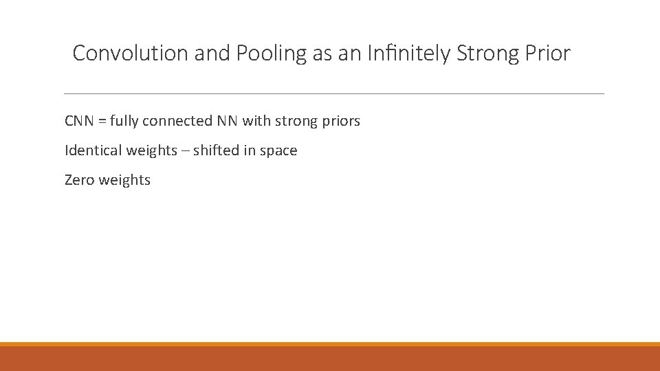
Convolution and Pooling as an Infinitely Strong Prior CNN = fully connected NN with strong priors Identical weights – shifted in space Zero weights

Convolution and Pooling as an Infinitely Strong Prior Key insights: 1. Convolution and pooling are only useful when the assumptions made by the prior are reasonably accurate. If not – may cause underfitting 2. We should only compare convolutional models to other convolutional models in benchmarks of statistical learning performance. Fully connected NN is permutation invariant.

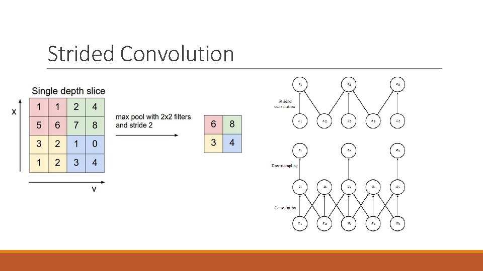
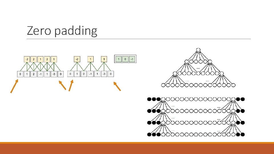
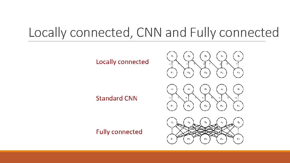
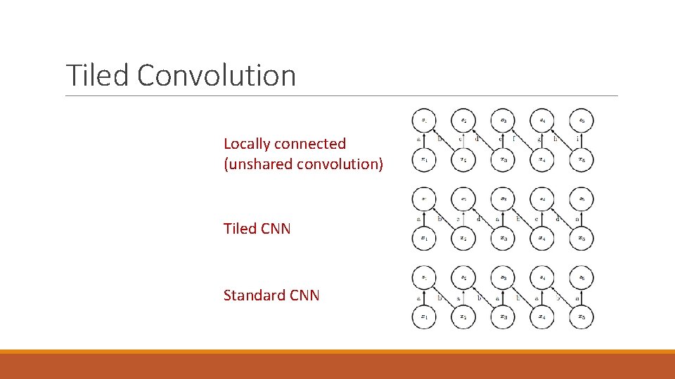
Variants of the Basic Convolution Function 1. Strided convolution 2. Zero padding 3. Unshared convolution 4. Tiled CNN

Strided Convolution

Zero padding

Locally connected, CNN and Fully connected Locally connected Standard CNN Fully connected

Tiled Convolution Locally connected (unshared convolution) Tiled CNN Standard CNN

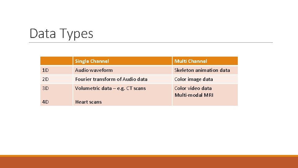
Data Types Single Channel Multi Channel 1 D Audio waveform Skeleton animation data 2 D Fourier transform of Audio data Color image data 3 D Volumetric data – e. g. CT scans 4 D Heart scans Color video data Multi-modal MRI

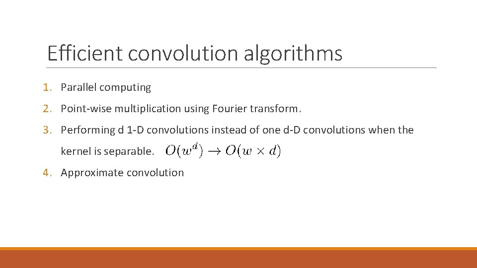
Efficient convolution algorithms 1. Parallel computing 2. Point-wise multiplication using Fourier transform. 3. Performing d 1 -D convolutions instead of one d-D convolutions when the kernel is separable. 4. Approximate convolution

Random or Unsupervised Features There a few basic strategies for obtaining convolution kernels without supervised training: 1. Random initialization 2. Design them by hand, for example by setting each kernel to detect edges at a certain orientation or scale. 3. Learn the kernels with an unsupervised criterion, For example, Coates et al. (2011) apply k-means clustering to small image patches, then use each learned centroid as a convolution kernel. 4. Unsupervised pre-training, One can then extract the features for the entire training set just once, essentially constructing a new training set for the last layer. Learning the last layer is then typically a convex optimization problem, assuming the last layer is something like logistic regression or an SVM.

Case studies (deeper, faster, stronger) 1. Le. Net - Le. Cun in 1990’s. 2. Alex. Net- Alex Krizhevsky, Ilya Sutskever and Geoff Hinton, Won Image. Net LSVRC challenge 2012 (like Le. Net but bigger and deeper) 3. ZF Net – M. Zeiler and R. Fergus ILSVRC 2013 winner (improving the Alex. Net by hyperparameter tweaking) 4. Goog. Le. Net- Szegedy et al. from Google, ILSVRC 2014 winner (Inception Module) 5. VGGNet – K. Simonyan and A. Zisserman runner-up in ILSVRC 2014 (depth matter) 6. Res. Net - Kaiming He et al, ILSVRC 2015 winner , special skip connections and a heavy use of batch normalization. 7. Image. Net Large Scale Visual Recognition Challenge (ILSVRC ) http: //imagenet. org/challenges/LSVRC/2016/