CSE 5542 Real Time Rendering Week 5 SlidesSome

CSE 5542 - Real Time Rendering Week 5

Slides(Some) Courtesy – E. Angel and D. Shreiner

Much Content …

What ? 4

Transformations

Where in Open. GL ?

In Vertex Shader

Typical Transform

Scaling

Scaling Expand or contract along each axis (fixed point of origin) x’=sxx y’=syx z’=szx p’=Sp S = S(sx, sy, sz) = 10

Linear Transform - Scaling

Scaling – This will do ! 2 x 2 3 x 3

As Matrices

Reflection corresponds to negative scale factors sx = -1 sy = 1 original sx = -1 sy = -1 sx = 1 sy = -1 14

Rotation

Rotation (2 D) Consider rotation about the origin by q degrees – radius stays the same, angle increases by q x = r cos (f + q) y = r sin (f + q) x’=x cos q –y sin q y’ = x sin q + y cos q x = r cos f y = r sin f 16

Rotation about z axis • Rotation about z axis in three dimensions leaves all points with the same z – Equivalent to rotation in two dimensions in planes of constant z x’=x cos q –y sin q y’ = x sin q + y cos q z’ =z – or in homogeneous coordinates p’=Rz(q)p 17

Rotation Matrix R = Rz(q) = 18

Example

X- & Y-axes Same argument as for rotation about z axis For rotation about x axis, x is unchanged For rotation about y axis, y is unchanged R = Rx(q) = Ry(q) = 20

Linear Spaces

Recap: Linear Independence A set of vectors v 1, v 2, …, vn is linearly independent if a 1 v 1+a 2 v 2+. . anvn=0 iff a 1=a 2=…=0 22

Recap: Coordinate Systems • • A basis v 1, v 2, …. , vn A vector is written v=a 1 v 1+ a 2 v 2 +…. +anvn Scalars {a 1, a 2, …. An}- representation of v given basis Representation as a row or column array of scalars a=[a 1 23 a 2 …. an]T=

Change of Coordinate System • Consider two representations of same vector with respect to two different bases: a=[a 1 a 2 a 3 ] b=[b 1 b 2 b 3] where v=a 1 v 1+ a 2 v 2 +a 3 v 3 = [a 1 a 2 a 3] [v 1 v 2 v 3] T =b u +b u = [b b b ] [u u u ] T 1 1 24 2 2 3 3 1 2 3

Second in Terms of First Each of the basis vectors, u 1, u 2, u 3, are vectors that can be represented in terms of the first basis u 1 = g 11 v 1+g 12 v 2+g 13 v 3 u 2 = g 21 v 1+g 22 v 2+g 23 v 3 u 3 = g 31 v 1+g 32 v 2+g 33 v 3 25 v

Recap: Matrix Form The coefficients define a 3 x 3 matrix M= and the bases can be related by a=MTb 26

Translation • Move (translate, displace) a point to a new location P’ d P • Displacement determined by a vector d – Three degrees of freedom – P’=P+d 27

Translating in 3 D object 28 translation: every point displaced by same vector

Translation

With 2 D/3 D Vectors

In Matrix Form

As Matrices

As Code

Homogenous Coordinates

Homogenous Coordinates

Allows Linearity

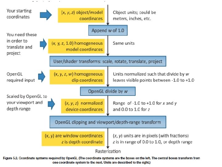
Homogeneous Coordinates Homogeneous coordinates for [x y z]: p =[x’ y’ z’ w] T =[wx wy wz w] T Three dimensional point (for w 0) by x x’/w, y y’/w, z z’/w If w=0, the representation is that of a vector Replaces points in 3 D by lines through origin in 4 D dimensions For w=1, the representation of a point is [x y z 1] 37

In Computer Graphics Homogeneous coordinates key – All standard transformations: rotation, translation, scaling. – Implemented matrix multiplications with 4 x 4 matrices – Hardware pipeline works with 4 D representations – Orthographic viewing: w=0 – vectors & w=1 – points – For perspective we need a perspective division 38

Recap: Frames • A coordinate system is insufficient for points • Origin & basis vectors form a frame v 2 P 0 v 3 39 v 1

Recap : Unified Representation • Frame determined by (P 0, v 1, v 2, v 3) • For this frame, every vector can be written as v=a 1 v 1+ a 2 v 2 +…. +anvn • Every point can be written as P = P 0 + b 1 v 1+ b 2 v 2 +…. +bnvn 40

Recap : Unified Representation Since 0 • P = 0 and 1 • P =P v=a 1 v 1+ a 2 v 2 +a 3 v 3 = [a 1 a 2 a 3 0 ] [v 1 v 2 v 3 P 0] T P = P 0 + b 1 v 1+ b 2 v 2 +b 3 v 3= [b 1 b 2 b 3 1 ] [v 1 v 2 v 3 P 0] T Thus we obtain the four-dimensional homogeneous coordinate representation v = [a 1 a 2 a 3 0 ] T p = [b 1 b 2 b 3 1 ] T 41

Change of Frames • We can apply a similar process in homogeneous coordinates to the representations of both points and vectors Consider two frames: (P 0, v 1, v 2, v 3) (Q 0, u 1, u 2, u 3) v 2 P 0 u 2 u 1 Q 0 v 1 u 3 v 3 • Any point or vector can be represented in either frame • We can represent Q 0, u 1, u 2, u 3 in terms of P 0, v 1, v 2, v 3 42

One Frame in Terms of Other Extending what we did with change of bases u 1 = g 11 v 1+g 12 v 2+g 13 v 3 u 2 = g 21 v 1+g 22 v 2+g 23 v 3 u 3 = g 31 v 1+g 32 v 2+g 33 v 3 Q 0 = g 41 v 1+g 42 v 2+g 43 v 3 +g 44 P 0 defining a 4 x 4 matrix M= 43

Working with Representations Within the two frames any point or vector has a representation of the same form a=[a 1 a 2 a 3 a 4 ] in the first frame b=[b 1 b 2 b 3 b 4 ] in the second frame where a 4 = b 4 = 1 for points and a 4 = b 4 = 0 for vectors and a=MTb The matrix M is 4 x 4 and specifies an affine transformation in homogeneous coordinates 44

Affine Transformations • Every linear transformation is equivalent to a change in frames • Every affine transformation preserves lines • However, an affine transformation has only 12 degrees of freedom because 4 of the elements in the matrix are fixed and are a subset of all possible 4 x 4 linear transformations 45

General Structure

Inverses • Can compute inverses use simple geometric observations – Translation: T-1(dx, dy, dz) = T(-dx, -dy, -dz) – Rotation: R -1(q) = R(-q) • Holds for any rotation matrix • Note that since cos(-q) = cos(q) and sin(-q)=-sin(q) R -1(q) = R T(q) – Scaling: S-1(sx, sy, sz) = S(1/sx, 1/sy, 1/sz) 47

Concatenation • We can form arbitrary affine transformation matrices by multiplying together rotation, translation, and scaling matrices • Since same transformation is applied to many vertices, the cost of forming a matrix M=ABCD is not significant compared to the cost of computing Mp for many vertices p 48

In-situ Transformations

In Place Scaling

As Opposed To

As Matrices and code

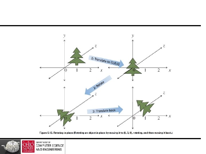
Fixed Point Other Than Origin Move fixed point to origin Rotate Move fixed point back M = T(pf) R(q) T(-pf) 54

Order of Transformations • Note that matrix on the right is the first applied • Mathematically, the following are equivalent p’ = ABCp = A(B(Cp)) • In terms of column matrices p’T = p. TCTBTAT 55

In Shaders uniform mat 4 View. T, View. R, Model. T, Model. R, Model. S, Project; in vec 4 Vertex; void main() { gl_Position = Project * Model. S * Model. R * Model. T * View. R * View. T * Vertex; }

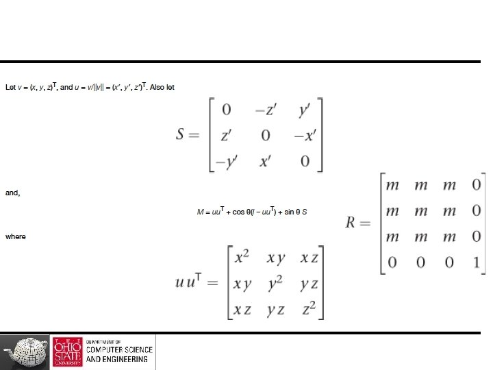
General Rotation About Origin A rotation by q about an arbitrary axis can be decomposed into the concatenation of rotations about the x, y, and z axes R(q) = Rz(qz) Ry(qy) Rx(qx) qx qy qz are called the Euler angles y Note that rotations do not commute We can use rotations in another order but with different angles 57 z q v x

Shear • Helpful to add one more basic transformation • Equivalent to pulling faces in opposite directions 59

Shear Matrix Consider simple shear along x axis x’ = x + y cot q y’ = y z’ = z H(q) = 60

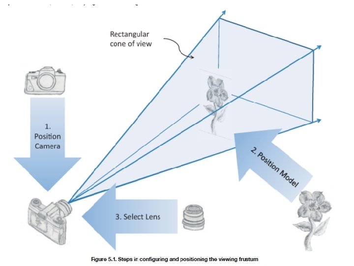
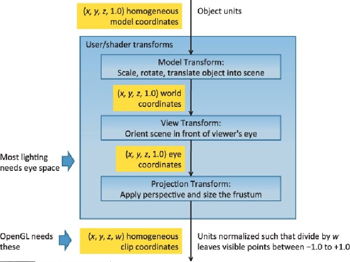
Viewing Transform

World & Camera Frames • Changes in frame are then defined by 4 x 4 matrices • In Open. GL, base frame is the world frame • Represent entities in the camera frame by changing world representation using model-view matrix • Initially these frames are the same (M=I) 62

Steps

Moving the Camera If objects are on both sides of z=0, move camera frame M= 65

Perspective P is defined as long as l ≠ r, t ≠ b, and n ≠ f.

Details

To Note z values will end up at 1. 0 ! Lose information about depth No scaling result to the [– 1. 0, 1. 0] range

Two Cases Symmetric, centered frustum, where z-axis is centered in the cone Asymmetric frustum- view thru a window and near it, but not toward its middle

Symmetric Case • Project points in frustum onto near plane • Line from (0, 0, 0) makes ratio of z to x same, and same for z to y for all points • xproj = x · znear, yproj = y · znear • Scale window size to [– 1. 0, 1. 0]

Symmetric Case

Asymmetric

Parallel Viewing P is defined as long as l ≠ r, t ≠ b, and n ≠ f.

Details

Symmetric

Asymmetric