CSA 3202 Human Language Technology HMMs for POS

CSA 3202 Human Language Technology HMMs for POS Tagging 1

Acknowledgement § Slides adapted from lecture by Dan Jurafsky

Hidden Markov Model Tagging § Using an HMM to do POS tagging is a special case of Bayesian inference § Foundational work in computational linguistics § Bledsoe 1959: OCR § Mosteller and Wallace 1964: authorship identification § It is also related to the “noisy channel” model that’s the basis for ASR, OCR and MT 3

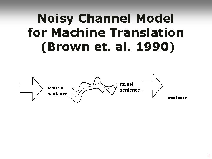
Noisy Channel Model for Machine Translation (Brown et. al. 1990) source sentence target sentence 4

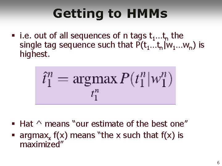
POS Tagging as Sequence Classification § Probabilistic view: § Given an observation sequence O = w 1…wn § e. g. Secretariat is expected to race tomorrow § What is the best sequence of tags T that corresponds to this sequence of observations? § Consider all possible sequences of tags § Out of this universe of sequences, choose the tag sequence which maximises P(T|O) 5

Getting to HMMs § i. e. out of all sequences of n tags t 1…tn the single tag sequence such that P(t 1…tn|w 1…wn) is highest. § Hat ^ means “our estimate of the best one” § argmaxx f(x) means “the x such that f(x) is maximized” 6

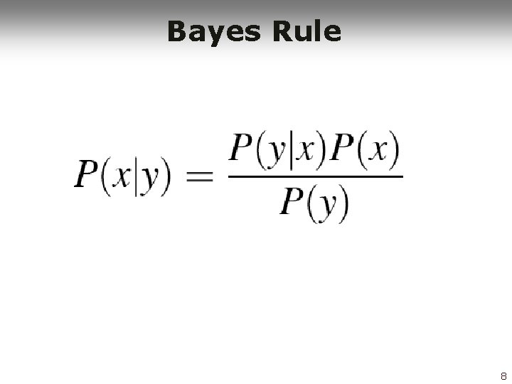
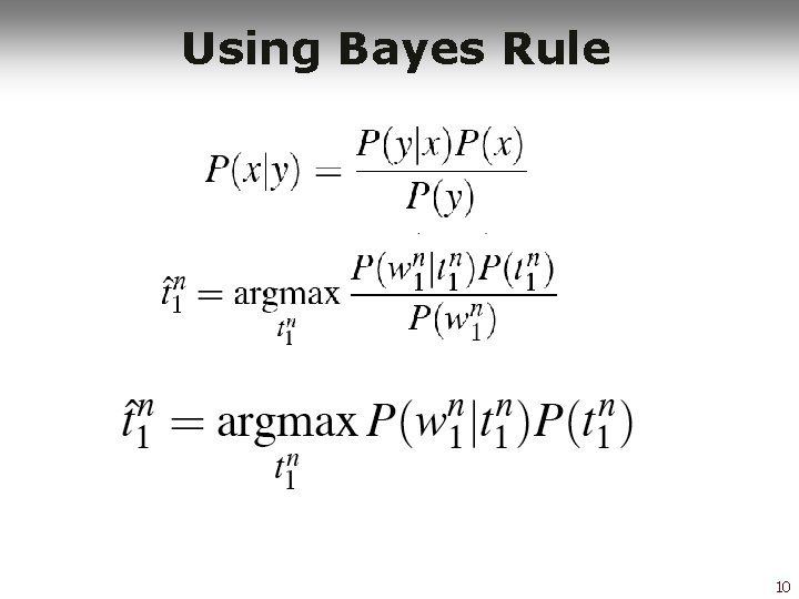
Getting to HMMs § But how to make it operational? How to compute this value? § Intuition of Bayesian classification: § Use Bayes Rule to transform this equation into a set of other probabilities that are easier to compute 7

Bayes Rule 8

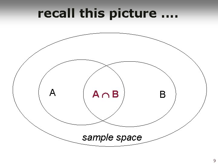
recall this picture. . A A B B sample space 9

Using Bayes Rule 10

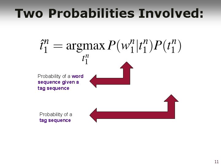
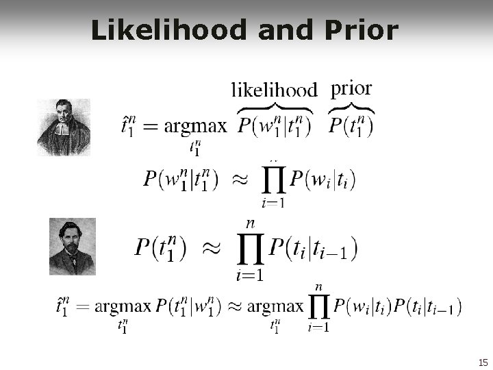
Two Probabilities Involved: Probability of a word sequence given a tag sequence Probability of a tag sequence 11

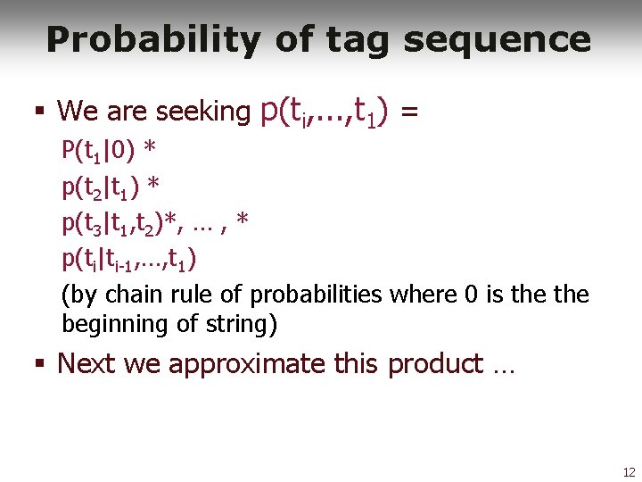
Probability of tag sequence § We are seeking p(ti, . . . , t 1) = P(t 1|0) * p(t 2|t 1) * p(t 3|t 1, t 2)*, … , * p(ti|ti-1, …, t 1) (by chain rule of probabilities where 0 is the beginning of string) § Next we approximate this product … 12

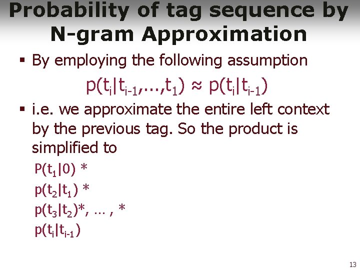
Probability of tag sequence by N-gram Approximation § By employing the following assumption p(ti|ti-1, . . . , t 1) ≈ p(ti|ti-1) § i. e. we approximate the entire left context by the previous tag. So the product is simplified to P(t 1|0) * p(t 2|t 1) * p(t 3|t 2)*, … , * p(ti|ti-1) 13

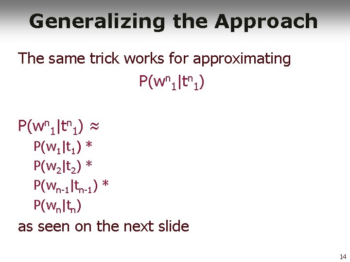
Generalizing the Approach The same trick works for approximating P(wn 1|tn 1) ≈ P(w 1|t 1) * P(w 2|t 2) * P(wn-1|tn-1) * P(wn|tn) as seen on the next slide 14

Likelihood and Prior 15

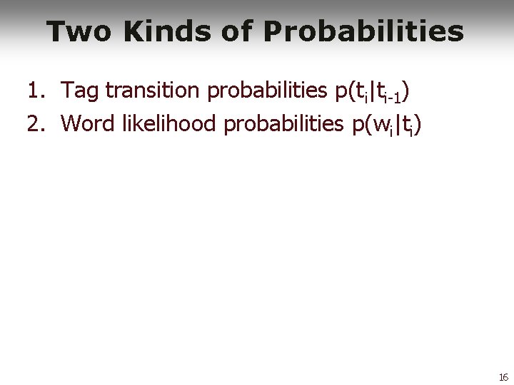
Two Kinds of Probabilities 1. Tag transition probabilities p(ti|ti-1) 2. Word likelihood probabilities p(wi|ti) 16

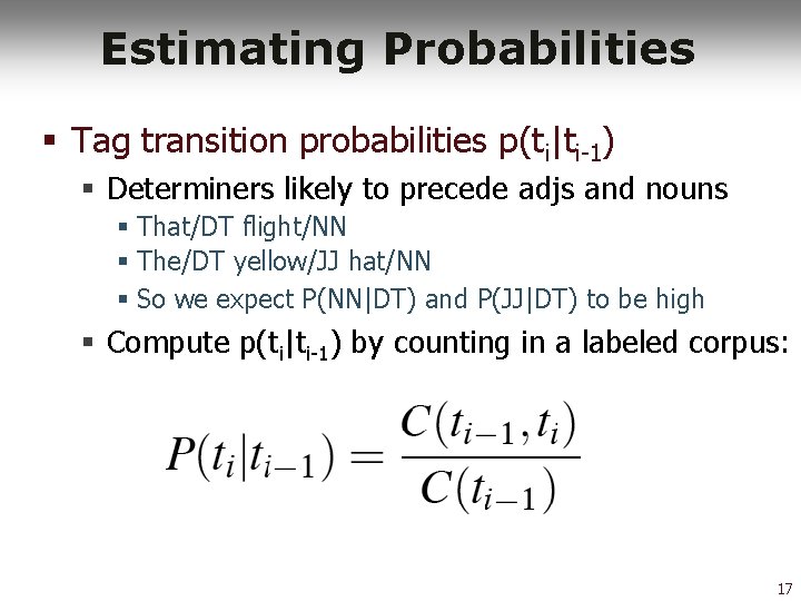
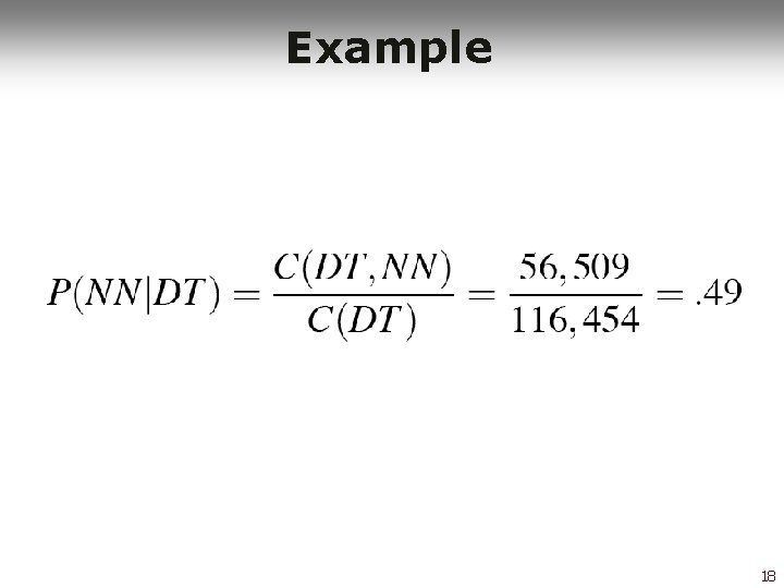
Estimating Probabilities § Tag transition probabilities p(ti|ti-1) § Determiners likely to precede adjs and nouns § That/DT flight/NN § The/DT yellow/JJ hat/NN § So we expect P(NN|DT) and P(JJ|DT) to be high § Compute p(ti|ti-1) by counting in a labeled corpus: 17

Example 18

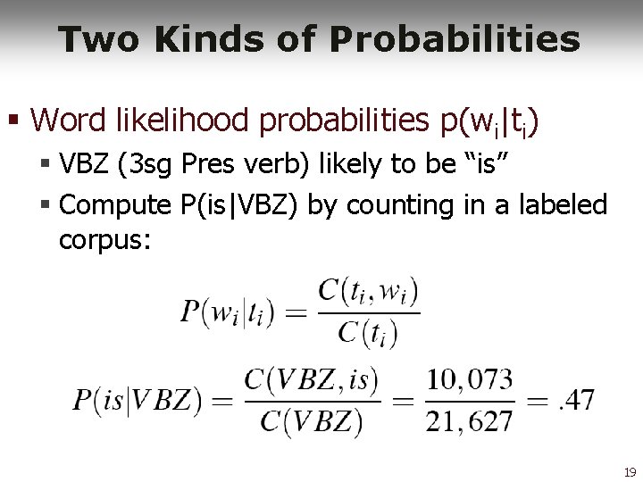
Two Kinds of Probabilities § Word likelihood probabilities p(wi|ti) § VBZ (3 sg Pres verb) likely to be “is” § Compute P(is|VBZ) by counting in a labeled corpus: 19

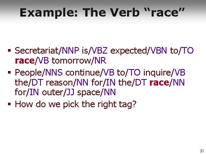
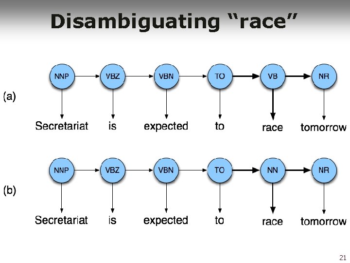
Example: The Verb “race” § Secretariat/NNP is/VBZ expected/VBN to/TO race/VB tomorrow/NR § People/NNS continue/VB to/TO inquire/VB the/DT reason/NN for/IN the/DT race/NN for/IN outer/JJ space/NN § How do we pick the right tag? 20

Disambiguating “race” 21

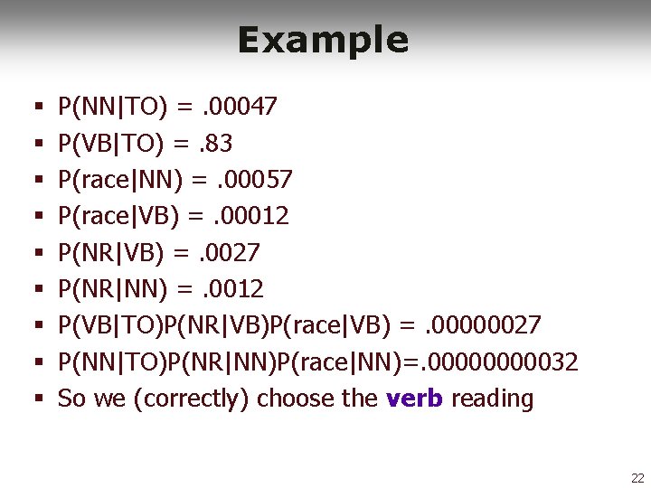
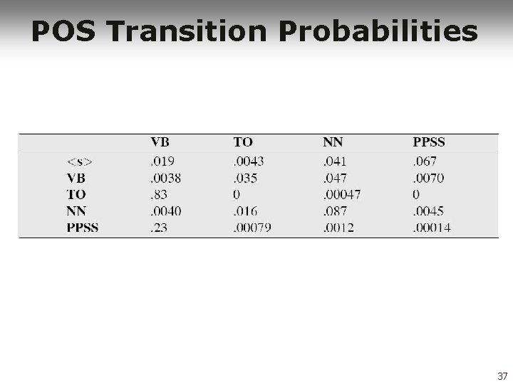
Example § § § § § P(NN|TO) =. 00047 P(VB|TO) =. 83 P(race|NN) =. 00057 P(race|VB) =. 00012 P(NR|VB) =. 0027 P(NR|NN) =. 0012 P(VB|TO)P(NR|VB)P(race|VB) =. 00000027 P(NN|TO)P(NR|NN)P(race|NN)=. 0000032 So we (correctly) choose the verb reading 22

Hidden Markov Models § What we’ve described with these two kinds of probabilities is a Hidden Markov Model (HMM) § We approach the concept of an HMM via the simpler notions § Weighted Finite State Automaton § Markov Chain 23

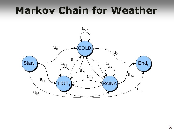
WFST Definition § A Weighted Finite-State Automaton (WFST) adds probabilities to the arcs § The sum of the probabilities leaving any arc must sum to one § A Markov chain is a special case of a WFST in which the input sequence uniquely determines which states the automaton will go through § Examples follow 24

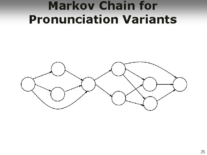
Markov Chain for Pronunciation Variants 25

Markov Chain for Weather 26

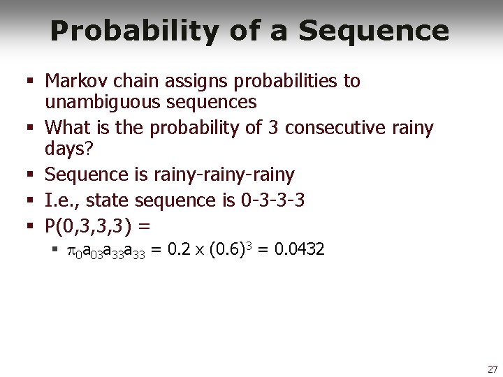
Probability of a Sequence § Markov chain assigns probabilities to unambiguous sequences § What is the probability of 3 consecutive rainy days? § Sequence is rainy-rainy § I. e. , state sequence is 0 -3 -3 -3 § P(0, 3, 3, 3) = § 0 a 03 a 33 = 0. 2 x (0. 6)3 = 0. 0432 27

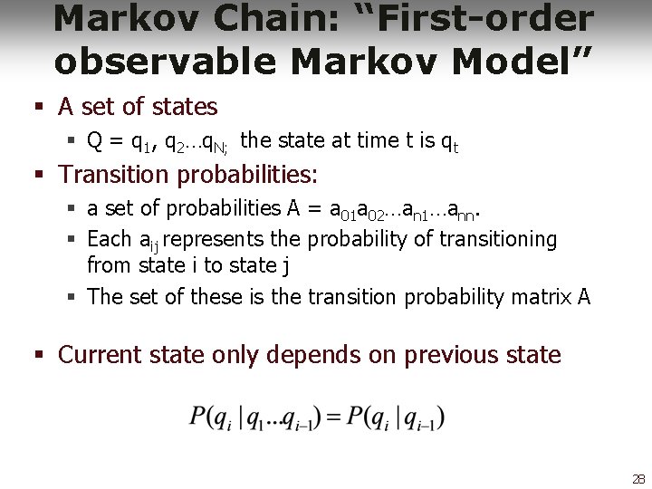
Markov Chain: “First-order observable Markov Model” § A set of states § Q = q 1, q 2…q. N; the state at time t is qt § Transition probabilities: § a set of probabilities A = a 01 a 02…an 1…ann. § Each aij represents the probability of transitioning from state i to state j § The set of these is the transition probability matrix A § Current state only depends on previous state 28

But. . § Markov chains can’t represent inherently ambiguous problems § For that we need a Hidden Markov Model 29

Hidden Markov Model § For Markov chains, the output symbols are the same as the states. § See hot weather: we’re in state hot § But in part-of-speech tagging (and other things) § The output symbols are words § But the hidden states are part-of-speech tags § So we need an extension! § A Hidden Markov Model is an extension of a Markov chain in which the input symbols are not the same as the states. § This means we don’t know which state we are in. 30

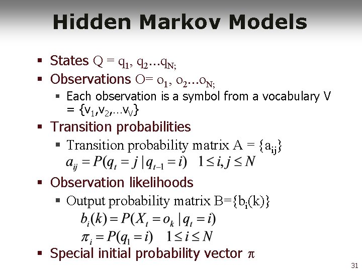
Hidden Markov Models § States Q = q 1, q 2…q. N; § Observations O= o 1, o 2…o. N; § Each observation is a symbol from a vocabulary V = {v 1, v 2, …v. V} § Transition probabilities § Transition probability matrix A = {aij} § Observation likelihoods § Output probability matrix B={bi(k)} § Special initial probability vector 31

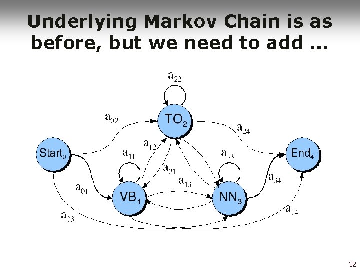
Underlying Markov Chain is as before, but we need to add. . . 32

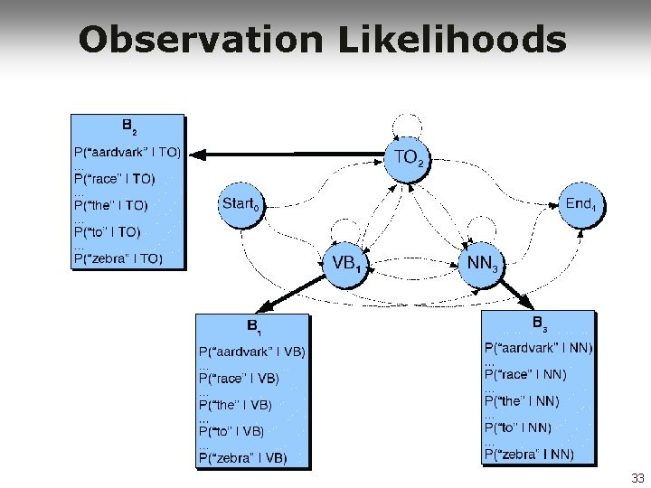
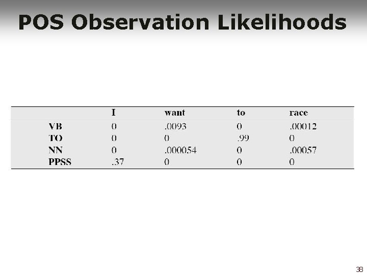
Observation Likelihoods 33

Observation Likelihoods § Observation likelihoods P(O|S) link actual observations O with underlying states S § Are necessary whenever there is not a 1: 1 correspondence between the two. § Examples from many different domains where there is uncertainty of interpretation § § OCR Speech Recognition Spelling Correction POS 34

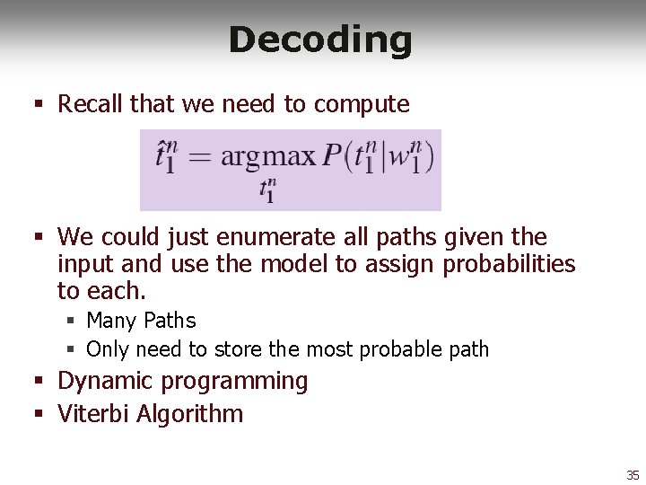
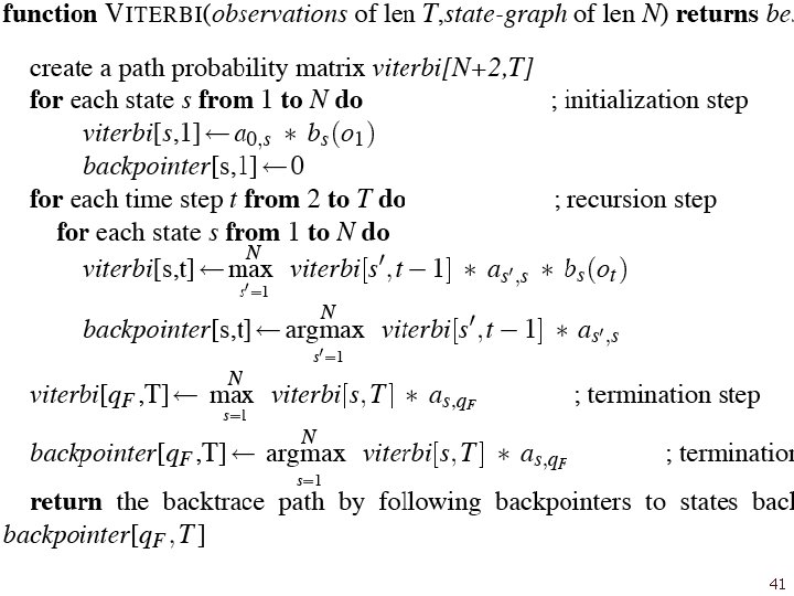
Decoding § Recall that we need to compute § We could just enumerate all paths given the input and use the model to assign probabilities to each. § Many Paths § Only need to store the most probable path § Dynamic programming § Viterbi Algorithm 35

Viterbi Algorithm § Inputs § HMM § Q: States § A: Transition probabilities § B: Observation likelihoods § O: Observed Words § Output § Most probable state/tag sequence together with its probability 36

POS Transition Probabilities 37

POS Observation Likelihoods 38

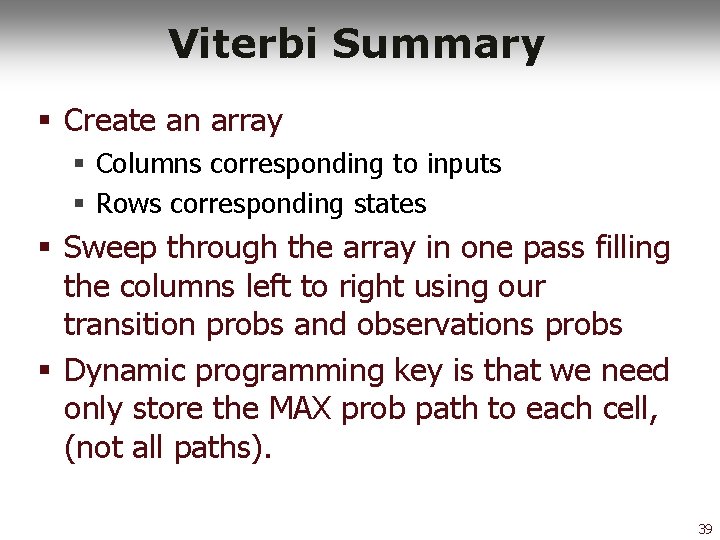
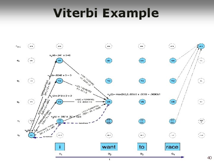
Viterbi Summary § Create an array § Columns corresponding to inputs § Rows corresponding states § Sweep through the array in one pass filling the columns left to right using our transition probs and observations probs § Dynamic programming key is that we need only store the MAX prob path to each cell, (not all paths). 39

Viterbi Example 40

41

POS-Tagger Evaluation § Different metrics can be used: § Overall error rate with respect to a goldstandard test set. § Error rates on particular tags c(gold(tok)=t and tagger(tok)=t)/ c(gold(tok)=t) § Error rates on particular words § Tag confusions. . . 42

Evaluation § The result is compared with a manually coded “Gold Standard” § Typically accuracy reaches 96 -97% § This may be compared with result for a baseline tagger (one that uses no context). § Important: 100% is impossible even for human annotators. § Inter annotator agreement problem 43

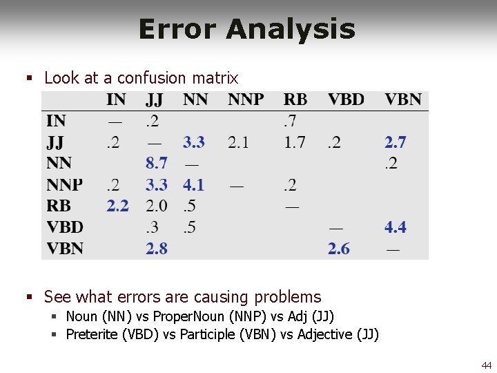
Error Analysis § Look at a confusion matrix § See what errors are causing problems § Noun (NN) vs Proper. Noun (NNP) vs Adj (JJ) § Preterite (VBD) vs Participle (VBN) vs Adjective (JJ) 44

POS Tagging Summary § Parts of speech § Tagsets § Part of speech tagging § Rule-Based § HMM Tagging § Markov Chains § Hidden Markov Models § Next: Transformation based 45