CS 473 Algorithms I SINGLESOURCE SHORTEST PATHS CS

CS 473 -Algorithms I SINGLE-SOURCE SHORTEST PATHS CS 473 Lecture. X 1

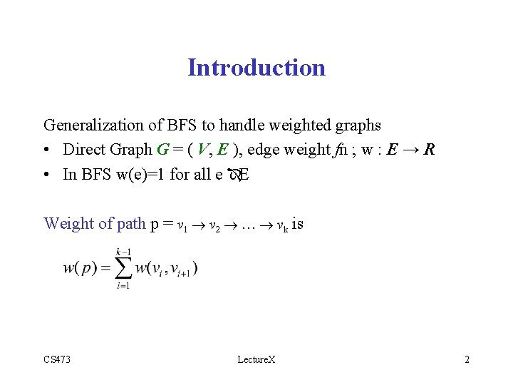
Introduction Generalization of BFS to handle weighted graphs • Direct Graph G = ( V, E ), edge weight fn ; w : E → R • In BFS w(e)=1 for all e ÎE Weight of path p = v 1 ® v 2 ® … ® vk is CS 473 Lecture. X 2

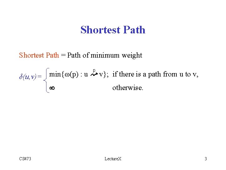
Shortest Path = Path of minimum weight δ(u, v)= min{ω(p) : u CS 473 p v}; if there is a path from u to v, otherwise. Lecture. X 3

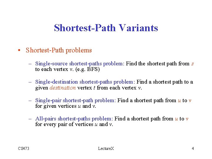
Shortest-Path Variants • Shortest-Path problems – Single-source shortest-paths problem: Find the shortest path from s to each vertex v. (e. g. BFS) – Single-destination shortest-paths problem: Find a shortest path to a given destination vertex t from each vertex v. – Single-pair shortest-path problem: Find a shortest path from u to v for given vertices u and v. – All-pairs shortest-paths problem: Find a shortest path from u to v for every pair of vertices u and v. CS 473 Lecture. X 4

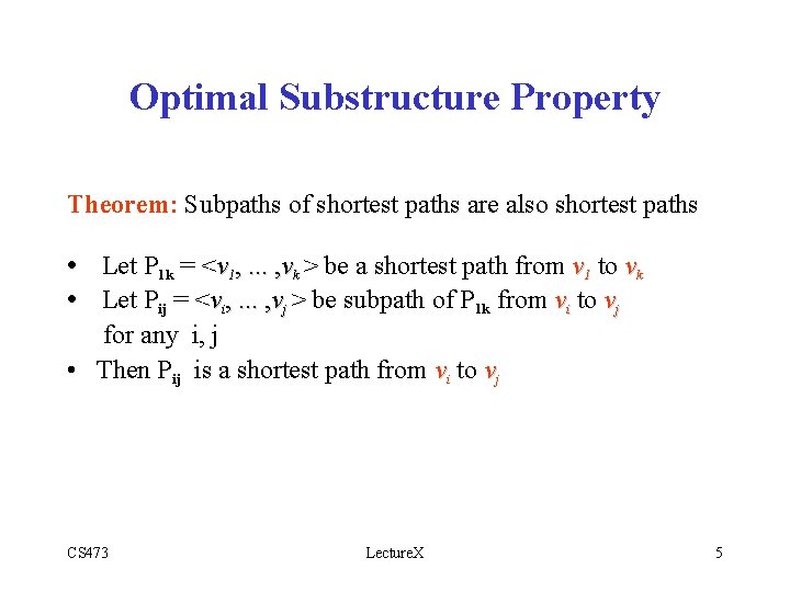
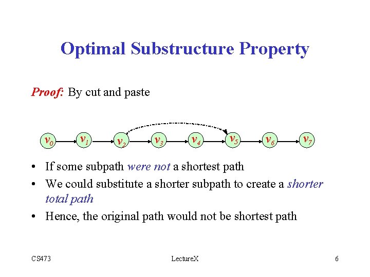
Optimal Substructure Property Theorem: Subpaths of shortest paths are also shortest paths • Let P 1 k = <v 1, . . . , vk > be a shortest path from v 1 to vk • Let Pij = <vi, . . . , vj > be subpath of P 1 k from vi to vj for any i, j • Then Pij is a shortest path from vi to vj CS 473 Lecture. X 5

Optimal Substructure Property Proof: By cut and paste v 0 v 1 v 2 v 3 v 4 v 5 v 6 v 7 • If some subpath were not a shortest path • We could substitute a shorter subpath to create a shorter total path • Hence, the original path would not be shortest path CS 473 Lecture. X 6

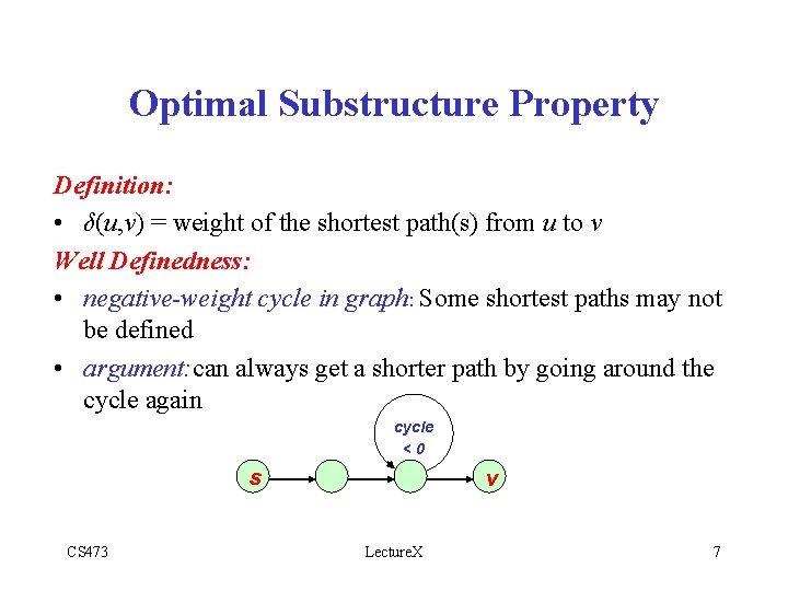
Optimal Substructure Property Definition: • δ(u, v) = weight of the shortest path(s) from u to v Well Definedness: • negative-weight cycle in graph: Some shortest paths may not be defined • argument: can always get a shorter path by going around the cycle again cycle <0 s CS 473 v Lecture. X 7

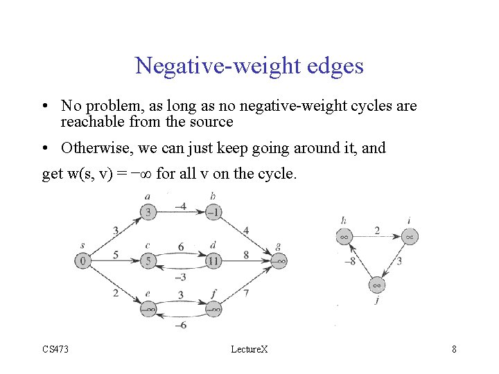
Negative-weight edges • No problem, as long as no negative-weight cycles are reachable from the source • Otherwise, we can just keep going around it, and get w(s, v) = −∞ for all v on the cycle. CS 473 Lecture. X 8

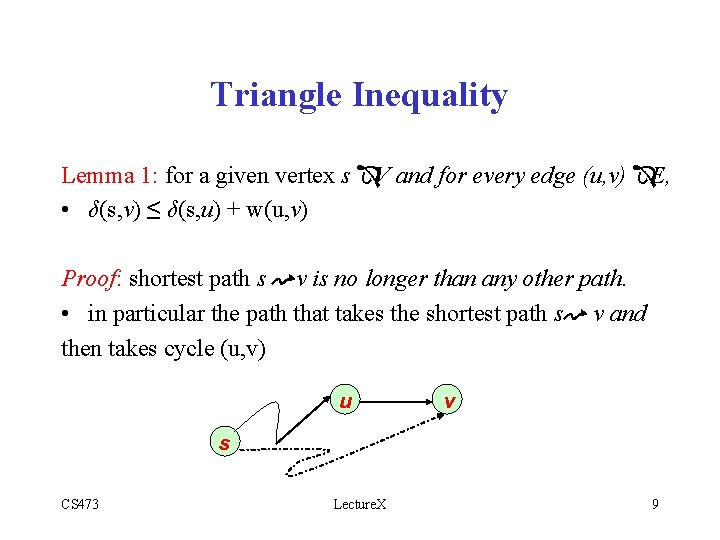
Triangle Inequality Lemma 1: for a given vertex s ÎV and for every edge (u, v) ÎE, • δ(s, v) ≤ δ(s, u) + w(u, v) Proof: shortest path s v is no longer than any other path. • in particular the path that takes the shortest path s v and then takes cycle (u, v) u v s CS 473 Lecture. X 9

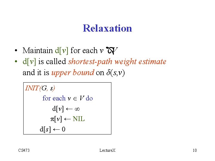
Relaxation • Maintain d[v] for each v ÎV • d[v] is called shortest-path weight estimate and it is upper bound on δ(s, v) INIT(G, s) for each v V do d[v] ← ∞ π[v] ← NIL d[s] ← 0 CS 473 Lecture. X 10

Relaxation RELAX(u, v) if d[v] > d[u]+w(u, v) then d[v] ← d[u]+w(u, v) π[v] ← u u 5 2 v u 9 5 2 v 6 Relax(u, v) 5 u CS 473 2 7 5 v u 2 6 v Lecture. X 11

Properties of Relaxation Algorithms differ in Ø how many times they relax each edge, and Ø the order in which they relax edges Question: How many times each edge is relaxed in BFS? Answer: Only once! CS 473 Lecture. X 12

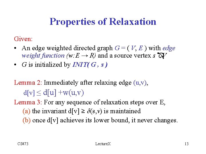
Properties of Relaxation Given: • An edge weighted directed graph G = ( V, E ) with edge weight function (w: E → R) and a source vertex s ÎV • G is initialized by INIT( G , s ) Lemma 2: Immediately after relaxing edge (u, v), d[v] ≤ d[u] +w(u, v) Lemma 3: For any sequence of relaxation steps over E, (a) the invariant d[v] ≥ δ(s, v) is maintained (b) once d[v] achieves its lower bound, it never changes. CS 473 Lecture. X 13

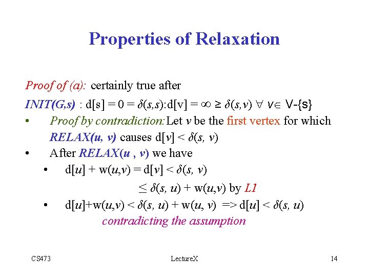
Properties of Relaxation Proof of (a): certainly true after INIT(G, s) : d[s] = 0 = δ(s, s): d[v] = ∞ ≥ δ(s, v) v V-{s} • Proof by contradiction: Let v be the first vertex for which RELAX(u, v) causes d[v] < δ(s, v) • After RELAX(u , v) we have • d[u] + w(u, v) = d[v] < δ(s, v) ≤ δ(s, u) + w(u, v) by L 1 • CS 473 d[u]+w(u, v) < δ(s, u) + w(u, v) => d[u] < δ(s, u) contradicting the assumption Lecture. X 14

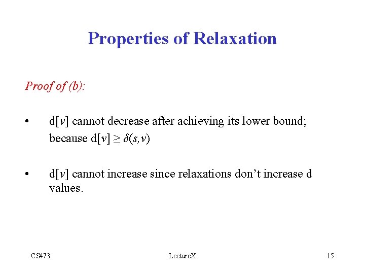
Properties of Relaxation Proof of (b): • d[v] cannot decrease after achieving its lower bound; because d[v] ≥ δ(s, v) • d[v] cannot increase since relaxations don’t increase d values. CS 473 Lecture. X 15

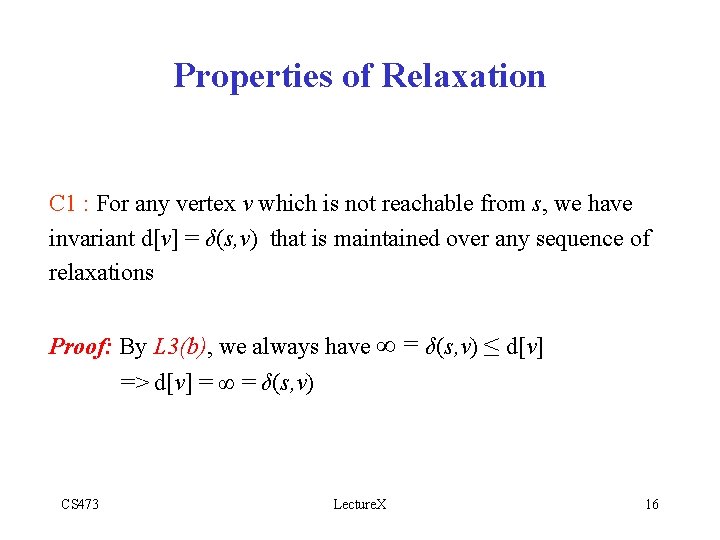
Properties of Relaxation C 1 : For any vertex v which is not reachable from s, we have invariant d[v] = δ(s, v) that is maintained over any sequence of relaxations Proof: By L 3(b), we always have ∞ = δ(s, v) ≤ d[v] => d[v] = ∞ = δ(s, v) CS 473 Lecture. X 16

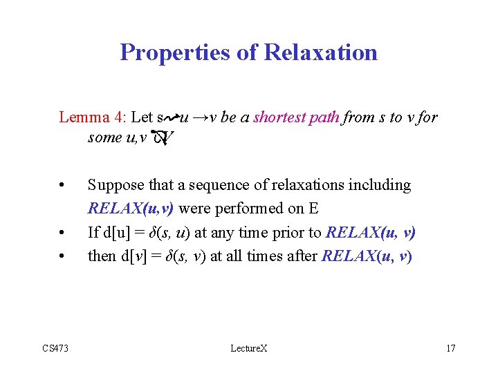
Properties of Relaxation Lemma 4: Let s u →v be a shortest path from s to v for some u, v ÎV • • • CS 473 Suppose that a sequence of relaxations including RELAX(u, v) were performed on E If d[u] = δ(s, u) at any time prior to RELAX(u, v) then d[v] = δ(s, v) at all times after RELAX(u, v) Lecture. X 17

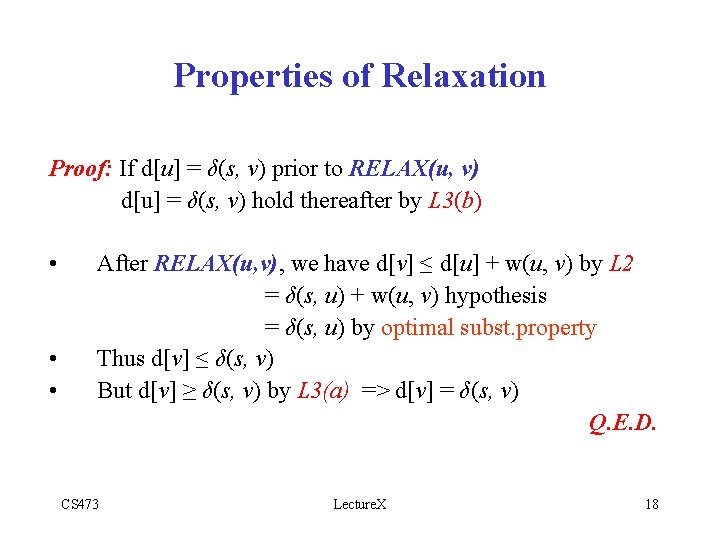
Properties of Relaxation Proof: If d[u] = δ(s, v) prior to RELAX(u, v) d[u] = δ(s, v) hold thereafter by L 3(b) • • • After RELAX(u, v), we have d[v] ≤ d[u] + w(u, v) by L 2 = δ(s, u) + w(u, v) hypothesis = δ(s, u) by optimal subst. property Thus d[v] ≤ δ(s, v) But d[v] ≥ δ(s, v) by L 3(a) => d[v] = δ(s, v) Q. E. D. CS 473 Lecture. X 18

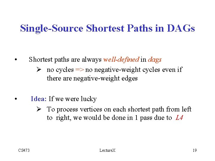
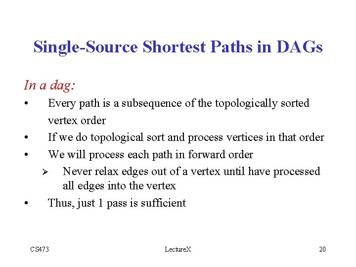
Single-Source Shortest Paths in DAGs • Shortest paths are always well-defined in dags Ø no cycles => no negative-weight cycles even if there are negative-weight edges • Idea: If we were lucky Ø To process vertices on each shortest path from left to right, we would be done in 1 pass due to L 4 CS 473 Lecture. X 19

Single-Source Shortest Paths in DAGs In a dag: • • Every path is a subsequence of the topologically sorted vertex order If we do topological sort and process vertices in that order We will process each path in forward order Ø Never relax edges out of a vertex until have processed all edges into the vertex Thus, just 1 pass is sufficient CS 473 Lecture. X 20

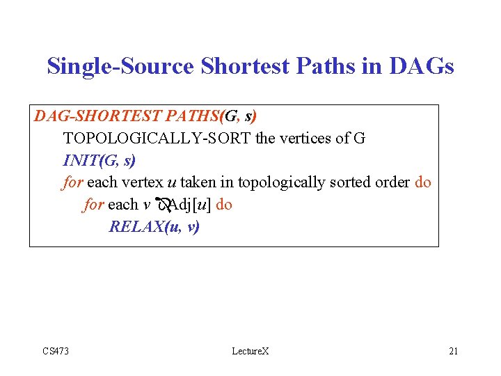
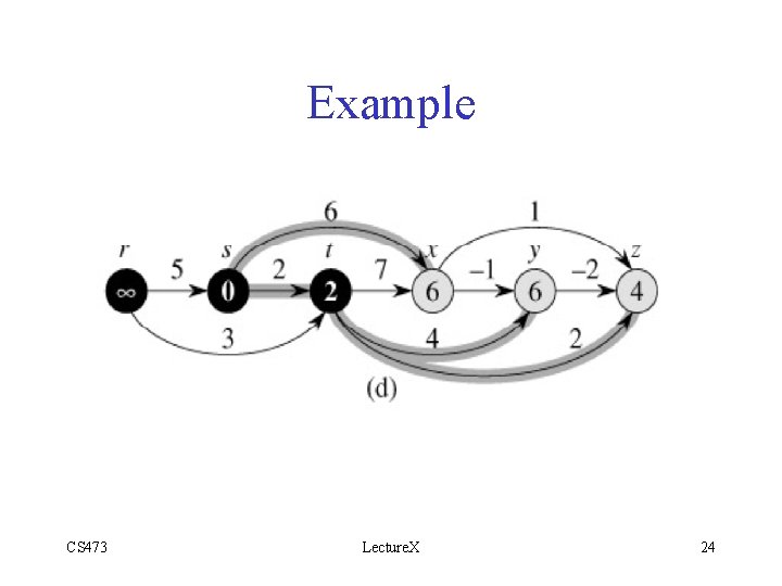
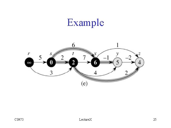
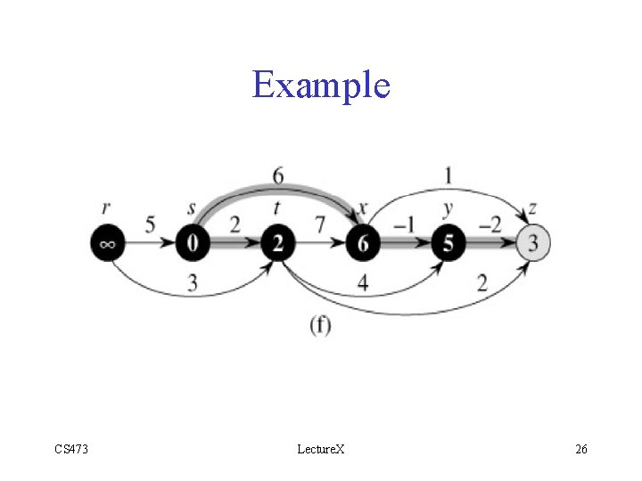
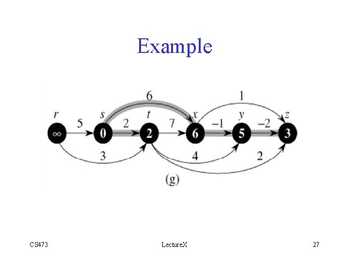
Single-Source Shortest Paths in DAGs DAG-SHORTEST PATHS(G, s) TOPOLOGICALLY-SORT the vertices of G INIT(G, s) for each vertex u taken in topologically sorted order do for each v ÎAdj[u] do RELAX(u, v) CS 473 Lecture. X 21

Example CS 473 Lecture. X 22

Example CS 473 Lecture. X 23

Example CS 473 Lecture. X 24

Example CS 473 Lecture. X 25

Example CS 473 Lecture. X 26

Example CS 473 Lecture. X 27

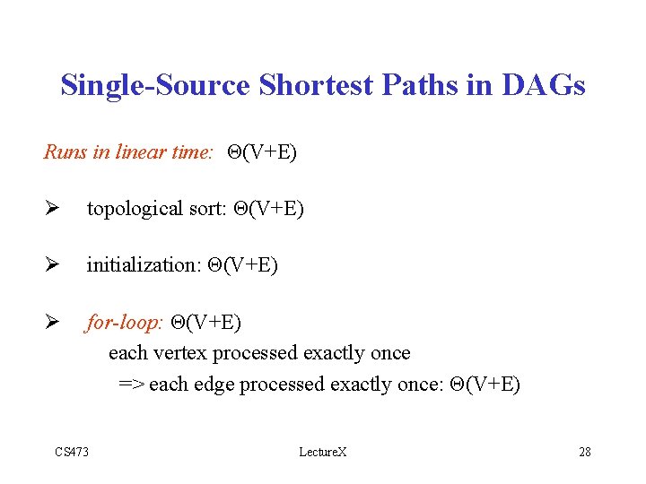
Single-Source Shortest Paths in DAGs Runs in linear time: Θ(V+E) Ø topological sort: Θ(V+E) Ø initialization: Θ(V+E) Ø for-loop: Θ(V+E) each vertex processed exactly once => each edge processed exactly once: Θ(V+E) CS 473 Lecture. X 28

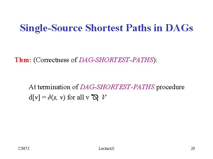
Single-Source Shortest Paths in DAGs Thm: (Correctness of DAG-SHORTEST-PATHS): At termination of DAG-SHORTEST-PATHS procedure d[v] = δ(s, v) for all v Î V CS 473 Lecture. X 29

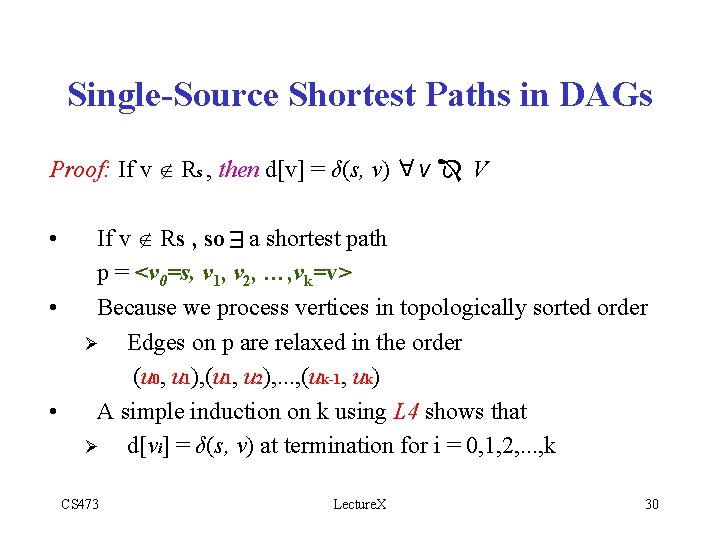
Single-Source Shortest Paths in DAGs • • vÎ V If v Rs , so a shortest path p = <v 0=s, v 1, v 2, …, vk=v> Because we process vertices in topologically sorted order Ø Edges on p are relaxed in the order (u 0, u 1), (u 1, u 2), . . . , (uk-1, uk) A simple induction on k using L 4 shows that Ø d[vi] = δ(s, v) at termination for i = 0, 1, 2, . . . , k E • A Proof: If v Rs , then d[v] = δ(s, v) CS 473 Lecture. X 30

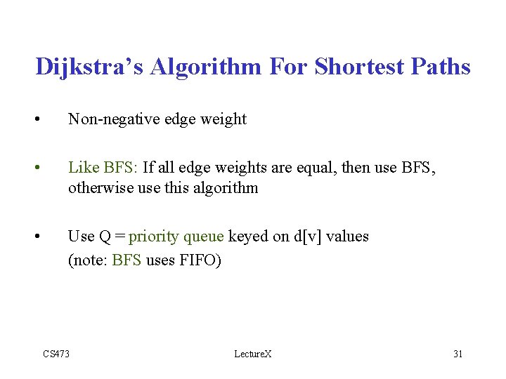
Dijkstra’s Algorithm For Shortest Paths • Non-negative edge weight • Like BFS: If all edge weights are equal, then use BFS, otherwise use this algorithm • Use Q = priority queue keyed on d[v] values (note: BFS uses FIFO) CS 473 Lecture. X 31

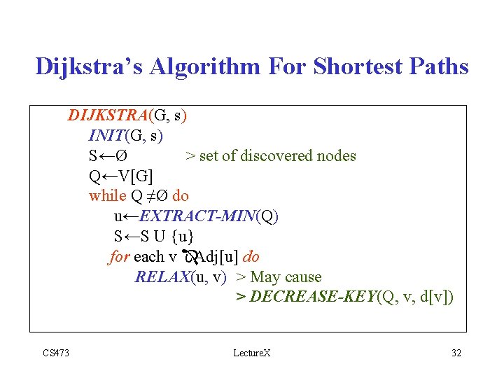
Dijkstra’s Algorithm For Shortest Paths DIJKSTRA(G, s) INIT(G, s) S←Ø > set of discovered nodes Q←V[G] while Q ≠Ø do u←EXTRACT-MIN(Q) S←S U {u} for each v ÎAdj[u] do RELAX(u, v) > May cause > DECREASE-KEY(Q, v, d[v]) CS 473 Lecture. X 32

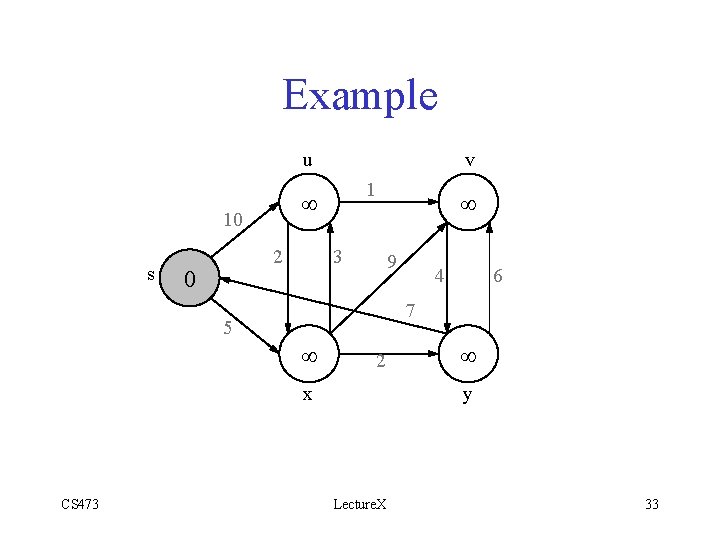
Example u 2 0 1 ¥ 10 s v 3 9 4 6 7 5 ¥ 2 x CS 473 ¥ ¥ y Lecture. X 33

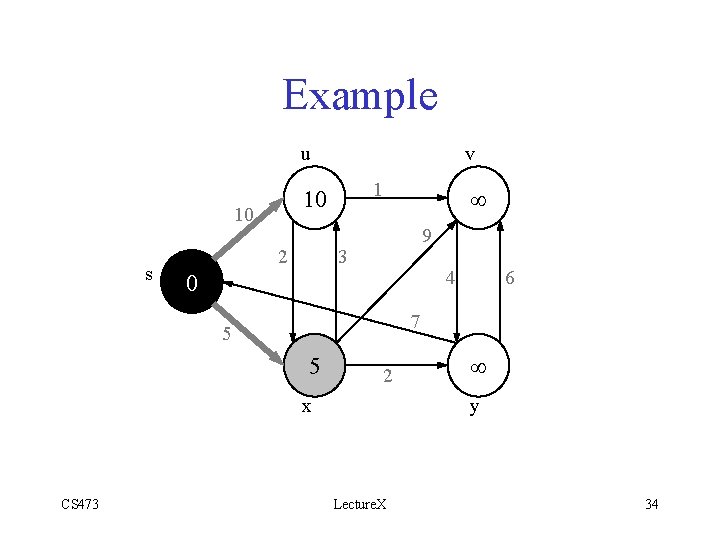
Example u 2 0 1 10 10 s v ¥ 9 3 4 7 5 5 2 x CS 473 6 ¥ y Lecture. X 34

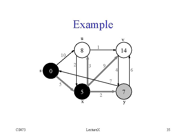
Example u 2 0 1 8 10 s v 14 9 3 6 7 5 5 2 x CS 473 4 7 y Lecture. X 35

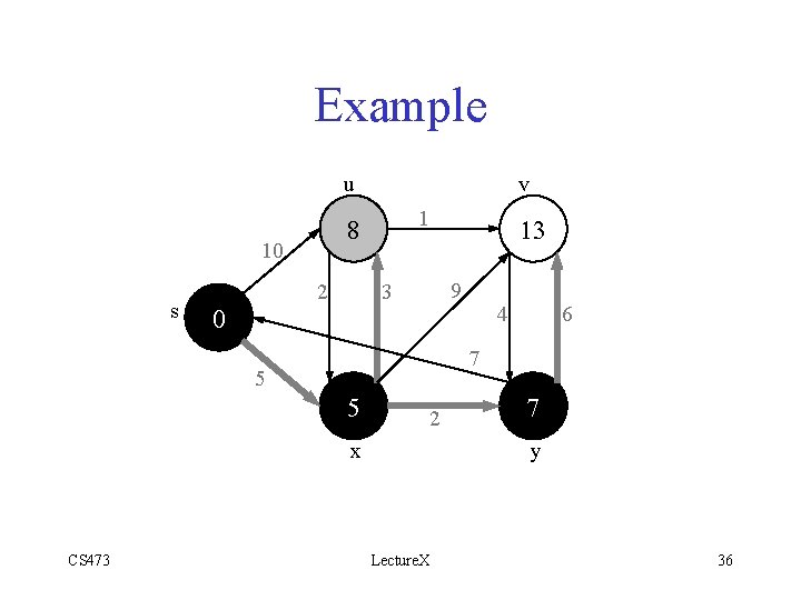
Example u 2 0 5 1 8 10 s v 13 9 3 6 7 5 2 x CS 473 4 7 y Lecture. X 36

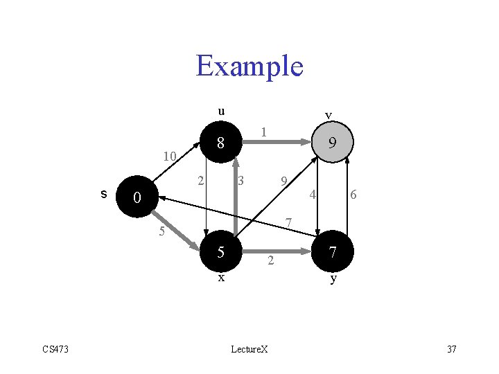
Example u 2 0 1 8 10 s v 9 3 9 6 7 5 5 2 x CS 473 4 7 y Lecture. X 37

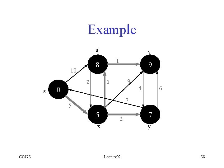
Example u 2 0 1 8 10 s v 9 9 3 4 7 5 5 2 x CS 473 6 7 y Lecture. X 38

Dijkstra’s Algorithm For Shortest Paths Observe : • • • Each vertex is extracted from Q and inserted into S exactly once Each edge is relaxed exactly once S = set of vertices whose final shortest paths have already been determined Ø i. e. , S = {v ÎV: d[v] = δ(s, v) ≠ ∞ } CS 473 Lecture. X 39

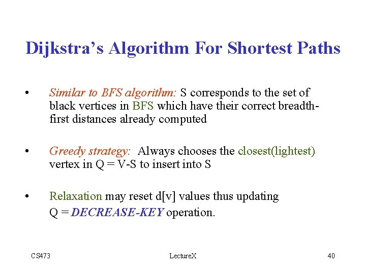
Dijkstra’s Algorithm For Shortest Paths • Similar to BFS algorithm: S corresponds to the set of black vertices in BFS which have their correct breadthfirst distances already computed • Greedy strategy: Always chooses the closest(lightest) vertex in Q = V-S to insert into S • Relaxation may reset d[v] values thus updating Q = DECREASE-KEY operation. CS 473 Lecture. X 40

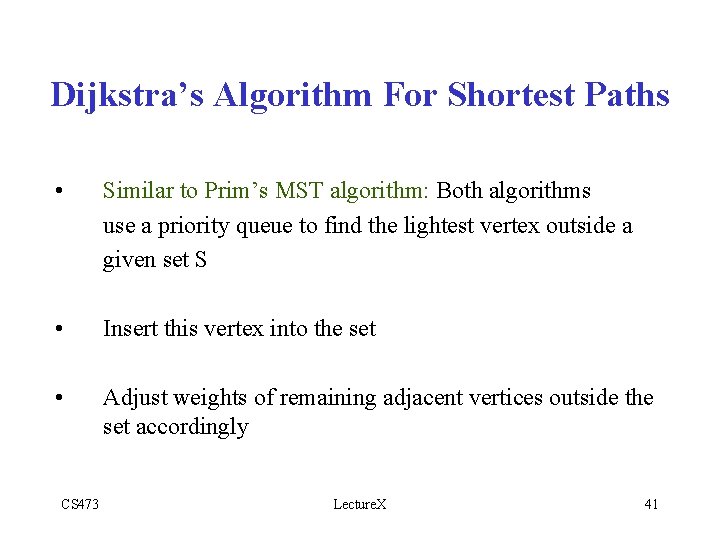
Dijkstra’s Algorithm For Shortest Paths • Similar to Prim’s MST algorithm: Both algorithms use a priority queue to find the lightest vertex outside a given set S • Insert this vertex into the set • Adjust weights of remaining adjacent vertices outside the set accordingly CS 473 Lecture. X 41

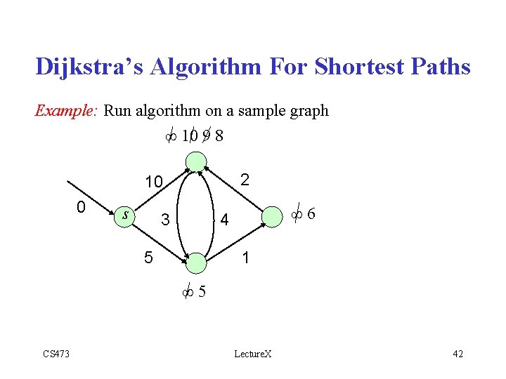
Dijkstra’s Algorithm For Shortest Paths Example: Run algorithm on a sample graph ∞ 10 9 8 2 10 0 s 3 ∞ 6 4 5 1 ∞ 5 CS 473 Lecture. X 42

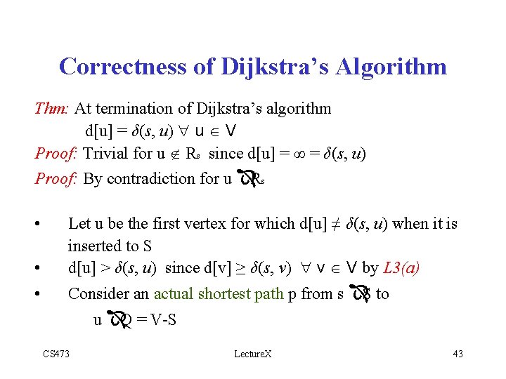
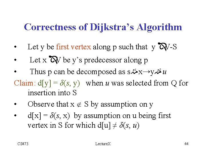
Correctness of Dijkstra’s Algorithm Thm: At termination of Dijkstra’s algorithm d[u] = δ(s, u) u V Proof: Trivial for u Rs since d[u] = ∞ = δ(s, u) Proof: By contradiction for u ÎRs • • • Let u be the first vertex for which d[u] ≠ δ(s, u) when it is inserted to S d[u] > δ(s, u) since d[v] ≥ δ(s, v) v V by L 3(a) Consider an actual shortest path p from s ÎS to u ÎQ = V-S CS 473 Lecture. X 43

Correctness of Dijkstra’s Algorithm • Let y be first vertex along p such that y ÎV-S • Let x ÎV be y’s predecessor along p • Thus p can be decomposed as s x→y p 2 u Claim: d[y] = δ(s, y) when u was selected from Q for insertion into S • Observe that x S by assumption on y • d[x] = δ(s, x) by assumption on u being first vertex in S for which d[u] ≠ δ(s, u) p 1 CS 473 Lecture. X 44

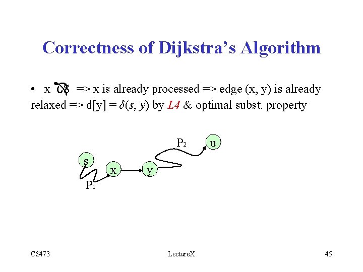
Correctness of Dijkstra’s Algorithm • x ÎS => x is already processed => edge (x, y) is already relaxed => d[y] = δ(s, y) by L 4 & optimal subst. property P 2 s x u y P 1 CS 473 Lecture. X 45

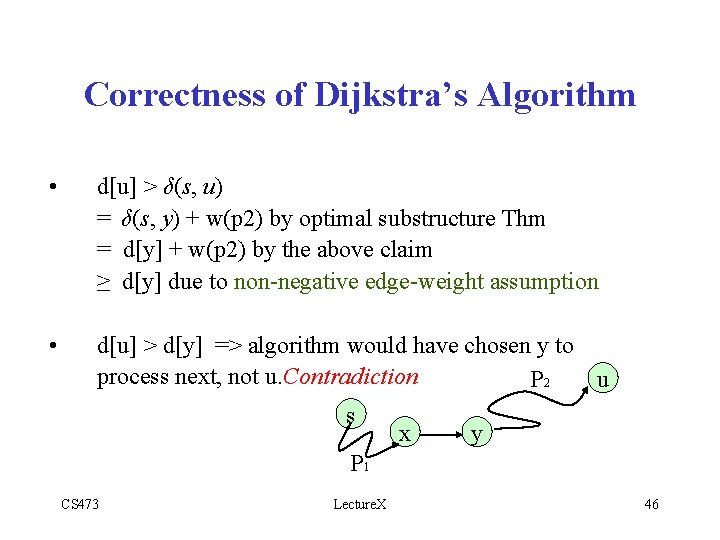
Correctness of Dijkstra’s Algorithm • d[u] > δ(s, u) = δ(s, y) + w(p 2) by optimal substructure Thm = d[y] + w(p 2) by the above claim ≥ d[y] due to non-negative edge-weight assumption • d[u] > d[y] => algorithm would have chosen y to process next, not u. Contradiction u P 2 s x y P 1 CS 473 Lecture. X 46

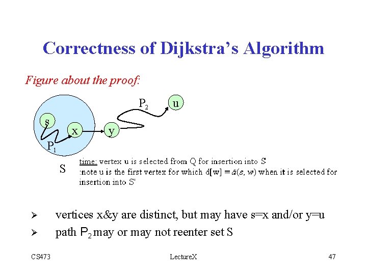
Correctness of Dijkstra’s Algorithm Figure about the proof: P 2 s x u y P 1 S Ø Ø CS 473 vertices x&y are distinct, but may have s=x and/or y=u path P 2 may or may not reenter set S Lecture. X 47

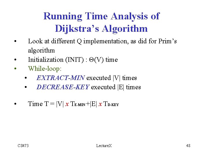
Running Time Analysis of Dijkstra’s Algorithm • • Look at different Q implementation, as did for Prim’s algorithm Initialization (INIT) : Θ(V) time While-loop: • EXTRACT-MIN executed |V| times • DECREASE-KEY executed |E| times Time T = |V| x TE-MIN +|E| x TD-KEY CS 473 Lecture. X 48

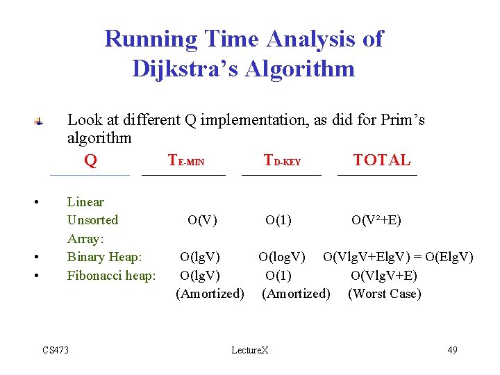
Running Time Analysis of Dijkstra’s Algorithm Look at different Q implementation, as did for Prim’s algorithm Q TE-MIN TD-KEY TOTAL • • • Linear Unsorted Array: Binary Heap: Fibonacci heap: CS 473 O(V) O(1) O(lg. V) (Amortized) O(V²+E) O(log. V) O(Vlg. V+Elg. V) = O(Elg. V) O(1) O(Vlg. V+E) (Amortized) (Worst Case) Lecture. X 49

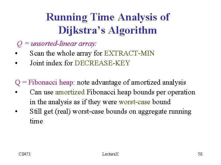
Running Time Analysis of Dijkstra’s Algorithm Q = unsorted-linear array: • Scan the whole array for EXTRACT-MIN • Joint index for DECREASE-KEY Q = Fibonacci heap: note advantage of amortized analysis • Can use amortized Fibonacci heap bounds per operation in the analysis as if they were worst-case bound • Still get (real) worst-case bounds on aggregate running time CS 473 Lecture. X 50

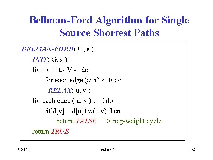
Bellman-Ford Algorithm for Single Source Shortest Paths • More general than Dijkstra’s algorithm: Ø Edge-weights can be negative • Detects the existence of negative-weight cycle(s) reachable from s. CS 473 Lecture. X 51

Bellman-Ford Algorithm for Single Source Shortest Paths BELMAN-FORD( G, s ) INIT( G, s ) for i ← 1 to |V|-1 do for each edge (u, v) E do RELAX( u, v ) for each edge ( u, v ) E do if d[v] > d[u]+w(u, v) then return FALSE > neg-weight cycle return TRUE CS 473 Lecture. X 52

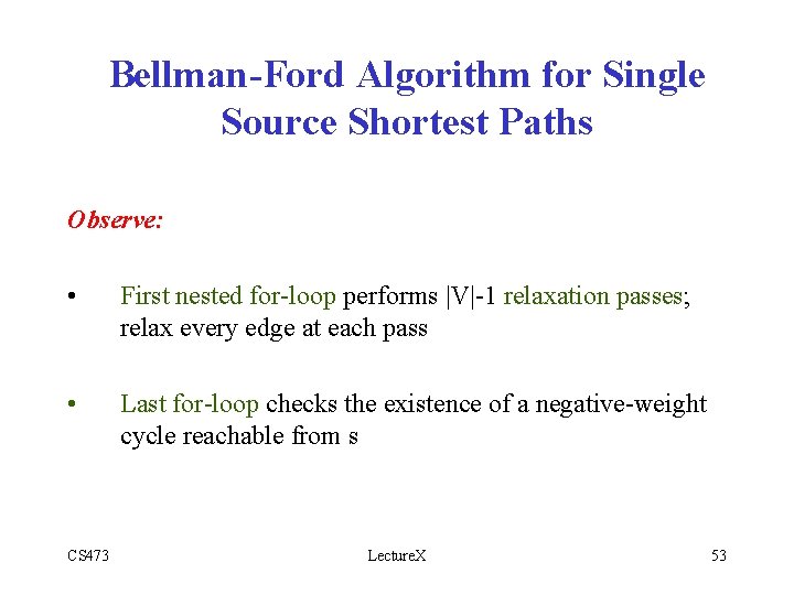
Bellman-Ford Algorithm for Single Source Shortest Paths Observe: • First nested for-loop performs |V|-1 relaxation passes; relax every edge at each pass • Last for-loop checks the existence of a negative-weight cycle reachable from s CS 473 Lecture. X 53

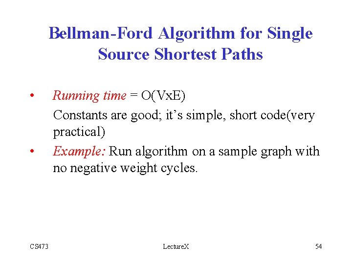
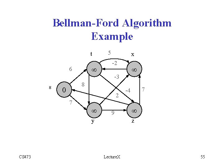
Bellman-Ford Algorithm for Single Source Shortest Paths • • CS 473 Running time = O(Vx. E) Constants are good; it’s simple, short code(very practical) Example: Run algorithm on a sample graph with no negative weight cycles. Lecture. X 54

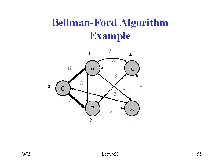
Bellman-Ford Algorithm Example t ¥ 6 s 5 x -2 -3 8 0 2 7 ¥ 9 y CS 473 ¥ 7 -4 ¥ z Lecture. X 55

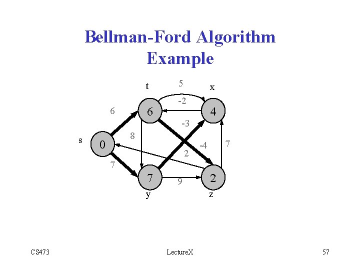
Bellman-Ford Algorithm Example 5 t 6 6 s x -2 -3 8 0 2 7 7 9 y CS 473 ¥ 7 -4 ¥ z Lecture. X 56

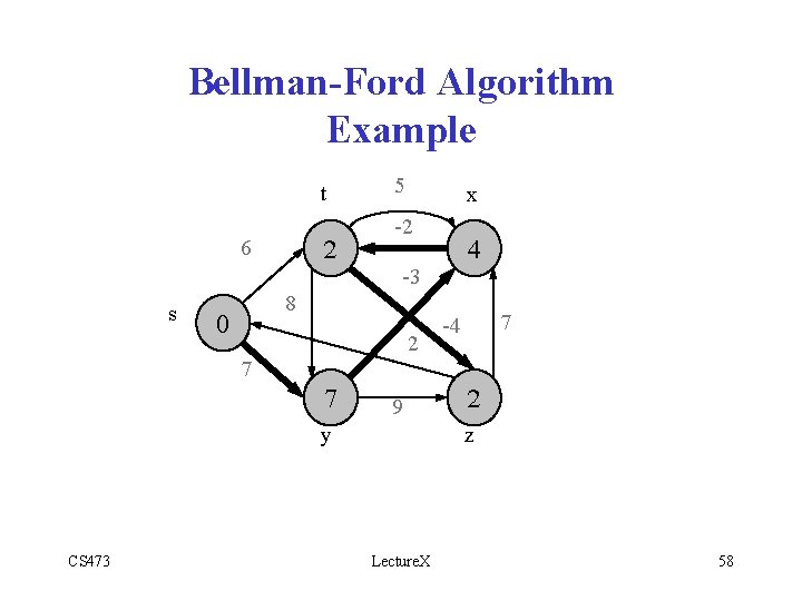
Bellman-Ford Algorithm Example t 6 6 s 5 x -2 -3 8 0 2 7 7 9 y CS 473 4 7 -4 2 z Lecture. X 57

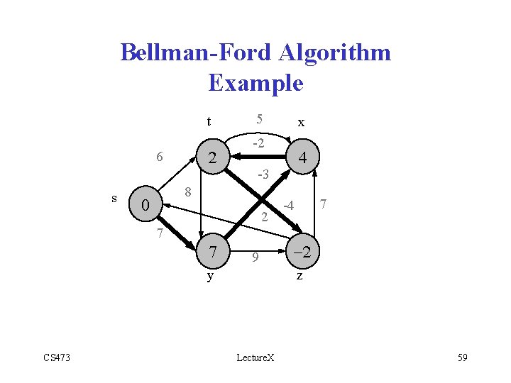
Bellman-Ford Algorithm Example t 2 6 s 5 x -2 -3 8 0 2 7 7 9 y CS 473 4 7 -4 2 z Lecture. X 58

Bellman-Ford Algorithm Example t 2 6 s 5 -2 2 7 7 9 y CS 473 4 -3 8 0 x 7 -4 -2 z Lecture. X 59

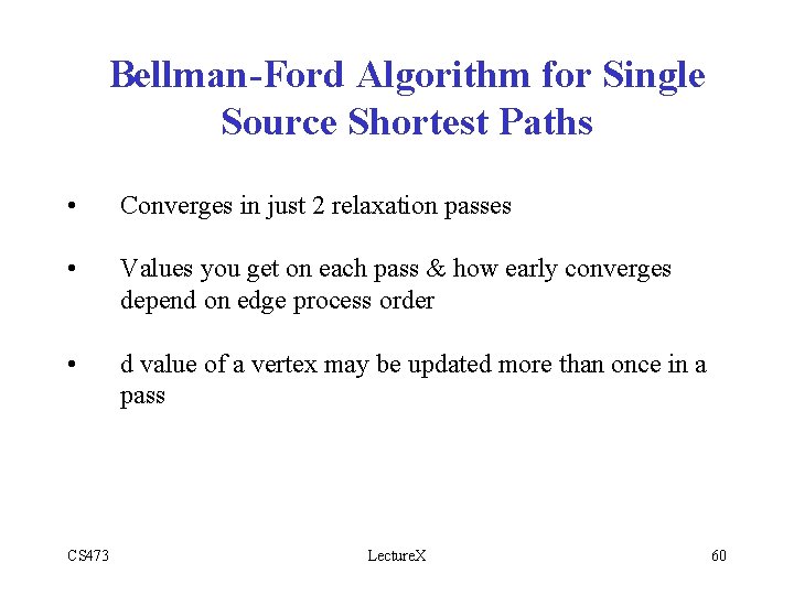
Bellman-Ford Algorithm for Single Source Shortest Paths • Converges in just 2 relaxation passes • Values you get on each pass & how early converges depend on edge process order • d value of a vertex may be updated more than once in a pass CS 473 Lecture. X 60

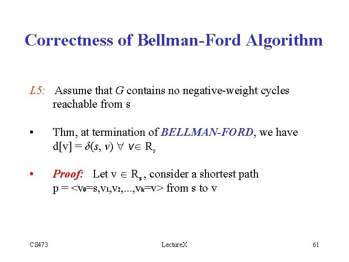
Correctness of Bellman-Ford Algorithm L 5: Assume that G contains no negative-weight cycles reachable from s • Thm, at termination of BELLMAN-FORD, we have d[v] = δ(s, v) v Rs • Proof: Let v Rs , consider a shortest path p = <v 0=s, v 1, v 2, . . . , vk=v> from s to v CS 473 Lecture. X 61

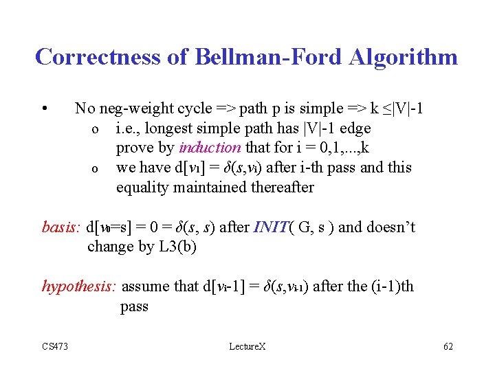
Correctness of Bellman-Ford Algorithm • No neg-weight cycle => path p is simple => k ≤|V|-1 o i. e. , longest simple path has |V|-1 edge prove by induction that for i = 0, 1, . . . , k o we have d[v 1] = δ(s, vi) after i-th pass and this equality maintained thereafter basis: d[v 0=s] = 0 = δ(s, s) after INIT( G, s ) and doesn’t change by L 3(b) hypothesis: assume that d[vi-1] = δ(s, vi-1) after the (i-1)th pass CS 473 Lecture. X 62

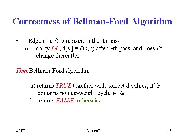
Correctness of Bellman-Ford Algorithm • Edge (vi-1, vi) is relaxed in the ith pass o so by L 4 , d[vi] = δ(s, vi) after i-th pass, and doesn’t change thereafter Thm: Bellman-Ford algorithm (a) returns TRUE together with correct d values, if G contains no neg-weight cycle Rs (b) returns FALSE, otherwise CS 473 Lecture. X 63

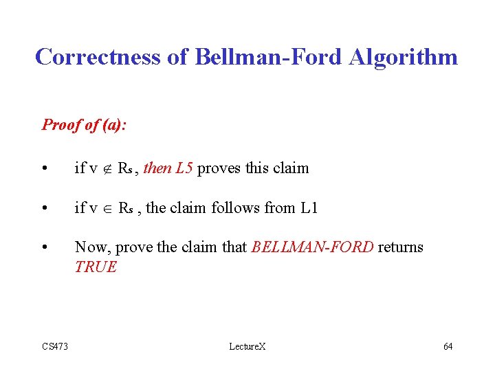
Correctness of Bellman-Ford Algorithm Proof of (a): • if v Rs , then L 5 proves this claim • if v Rs , the claim follows from L 1 • Now, prove the claim that BELLMAN-FORD returns TRUE CS 473 Lecture. X 64

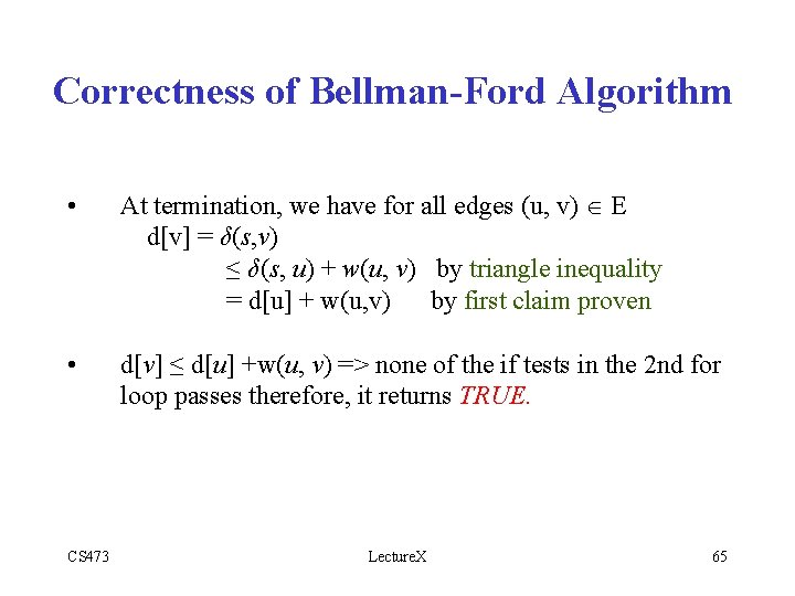
Correctness of Bellman-Ford Algorithm • At termination, we have for all edges (u, v) E d[v] = δ(s, v) ≤ δ(s, u) + w(u, v) by triangle inequality = d[u] + w(u, v) by first claim proven • d[v] ≤ d[u] +w(u, v) => none of the if tests in the 2 nd for loop passes therefore, it returns TRUE. CS 473 Lecture. X 65

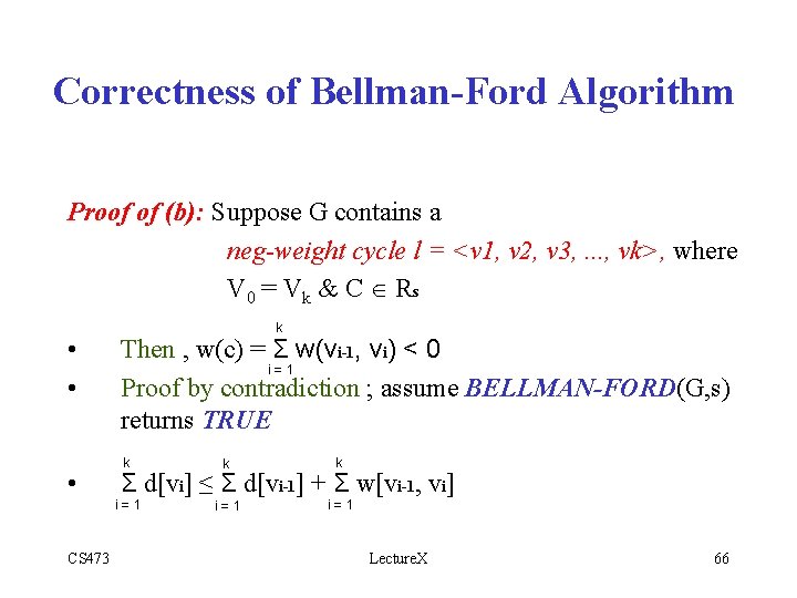
Correctness of Bellman-Ford Algorithm Proof of (b): Suppose G contains a neg-weight cycle l = <v 1, v 2, v 3, . . . , vk>, where V 0 = Vk & C R s • • • CS 473 k Then , w(c) = Σ w(vi-1, vi) < 0 i=1 Proof by contradiction ; assume BELLMAN-FORD(G, s) returns TRUE k k k i=1 i=1 Σ d[vi] ≤ Σ d[vi-1] + Σ w[vi-1, vi] Lecture. X 66

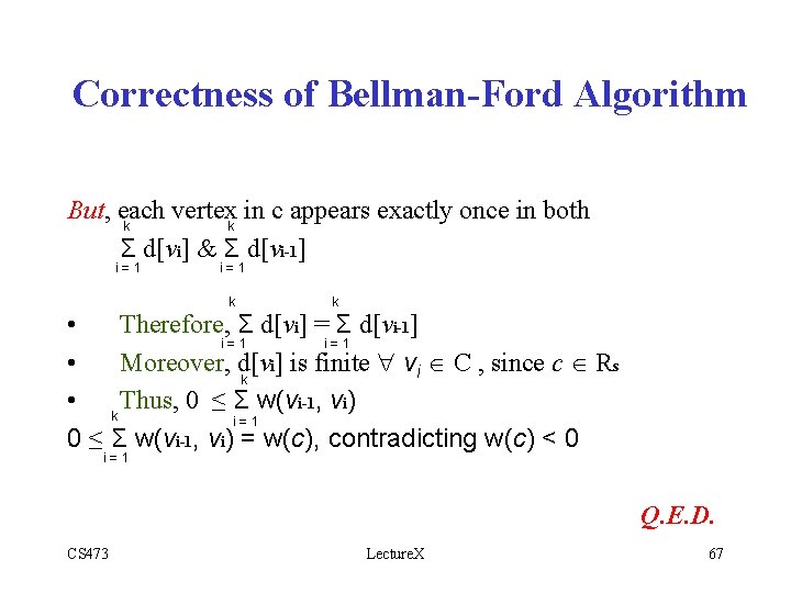
Correctness of Bellman-Ford Algorithm But, each vertexk in c appears exactly once in both k Σ d[vi] & Σ d[vi-1] i=1 k k • Therefore, Σ d[vi] = Σ d[vi-1] i=1 • Moreover, d[vi] is finite vi C , since c Rs k • k Thus, 0 ≤ Σ w(vi-1, vi) i=1 0 ≤ Σ w(vi-1, vi) = w(c), contradicting w(c) < 0 i=1 Q. E. D. CS 473 Lecture. X 67

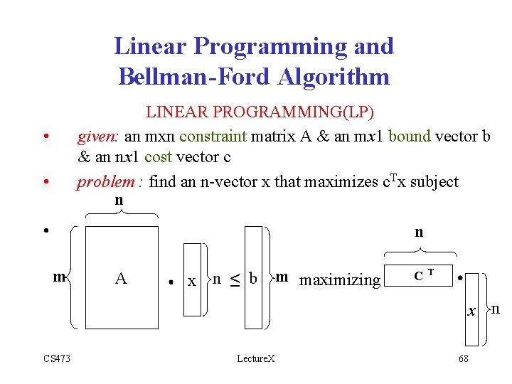
Linear Programming and Bellman-Ford Algorithm LINEAR PROGRAMMING(LP) given: an mxn constraint matrix A & an mx 1 bound vector b & an nx 1 cost vector c problem : find an n-vector x that maximizes c. Tx subject n • • • n m AA x n ≤ b m maximizing C T x n CS 473 Lecture. X 68

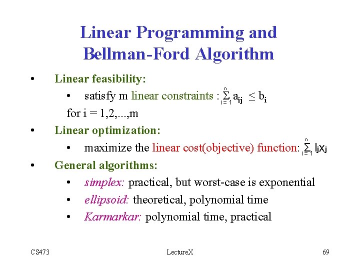
Linear Programming and Bellman-Ford Algorithm • • • CS 473 Linear feasibility: n • satisfy m linear constraints : i Σ a ≤ bi = 1 ij for i = 1, 2, . . . , m Linear optimization: n • maximize the linear cost(objective) function: i Σ ljxj =1 General algorithms: • simplex: practical, but worst-case is exponential • ellipsoid: theoretical, polynomial time • Karmarkar: polynomial time, practical Lecture. X 69

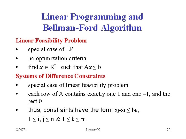
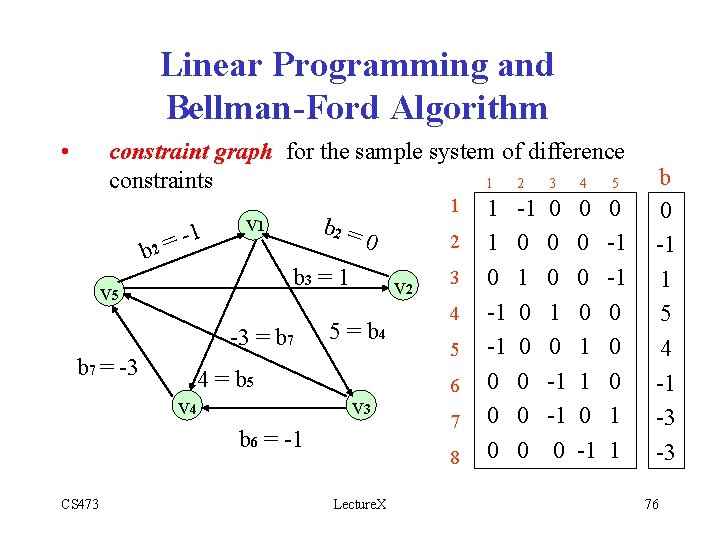
Linear Programming and Bellman-Ford Algorithm Linear Feasibility Problem • special case of LP • no optimization criteria • find x R n such that Ax ≤ b Systems of Difference Constraints • special case of linear feasibility problem • each row of A contains exactly one 1 and one – 1, and the rest 0 • thus, constraints have the form xj-xi ≤ bk , 1 ≤ i, j ≤ n & 1 ≤ k ≤ m CS 473 Lecture. X 70

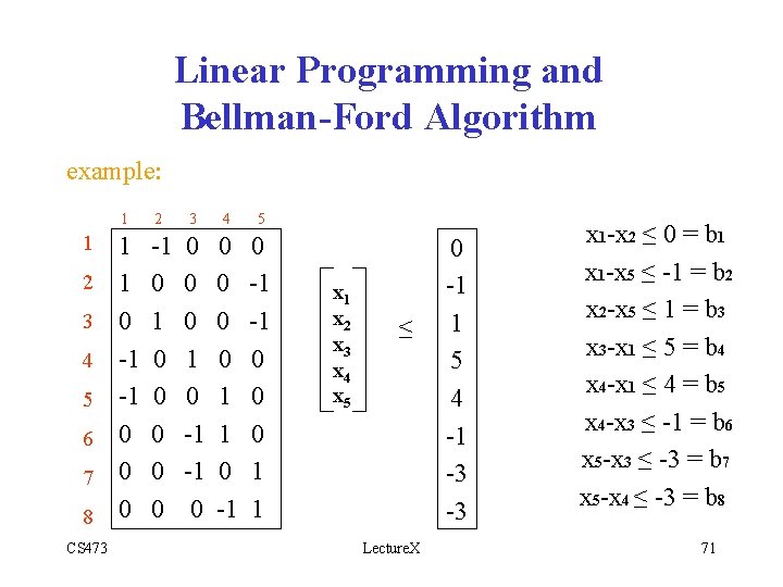
Linear Programming and Bellman-Ford Algorithm example: 1 2 3 4 5 6 7 8 CS 473 1 2 3 4 5 1 1 0 -1 -1 0 0 0 0 0 1 0 -1 -1 0 0 0 1 1 x 2 x 3 x 4 x 5 ≤ Lecture. X 0 -1 1 5 4 -1 -3 -3 x 1 -x 2 ≤ 0 = b 1 x 1 -x 5 ≤ -1 = b 2 x 2 -x 5 ≤ 1 = b 3 x 3 -x 1 ≤ 5 = b 4 x 4 -x 1 ≤ 4 = b 5 x 4 -x 3 ≤ -1 = b 6 x 5 -x 3 ≤ -3 = b 7 x 5 -x 4 ≤ -3 = b 8 71

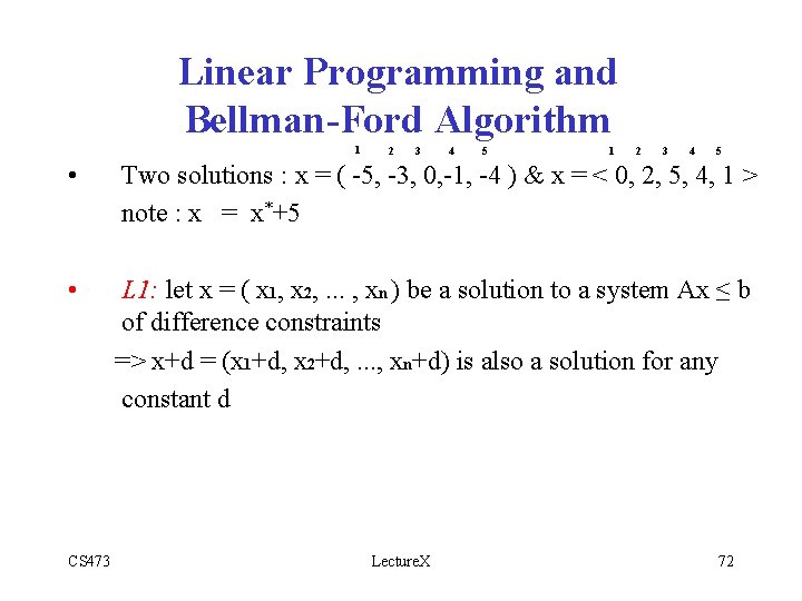
Linear Programming and Bellman-Ford Algorithm 1 2 3 4 5 • Two solutions : x = ( -5, -3, 0, -1, -4 ) & x = < 0, 2, 5, 4, 1 > note : x = x*+5 • L 1: let x = ( x 1, x 2, . . . , xn ) be a solution to a system Ax ≤ b of difference constraints => x+d = (x 1+d, x 2+d, . . . , xn+d) is also a solution for any constant d CS 473 Lecture. X 72

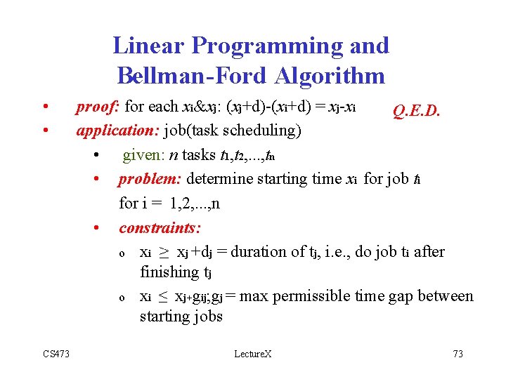
Linear Programming and Bellman-Ford Algorithm • • CS 473 proof: for each xi&xj: (xj+d)-(xi+d) = xj-xi Q. E. D. application: job(task scheduling) • given: n tasks t 1, t 2, . . . , tn • problem: determine starting time xi for job ti for i = 1, 2, . . . , n • constraints: o xi ≥ xj +dj = duration of tj, i. e. , do job ti after finishing tj o xi ≤ xj+gij; gj = max permissible time gap between starting jobs Lecture. X 73

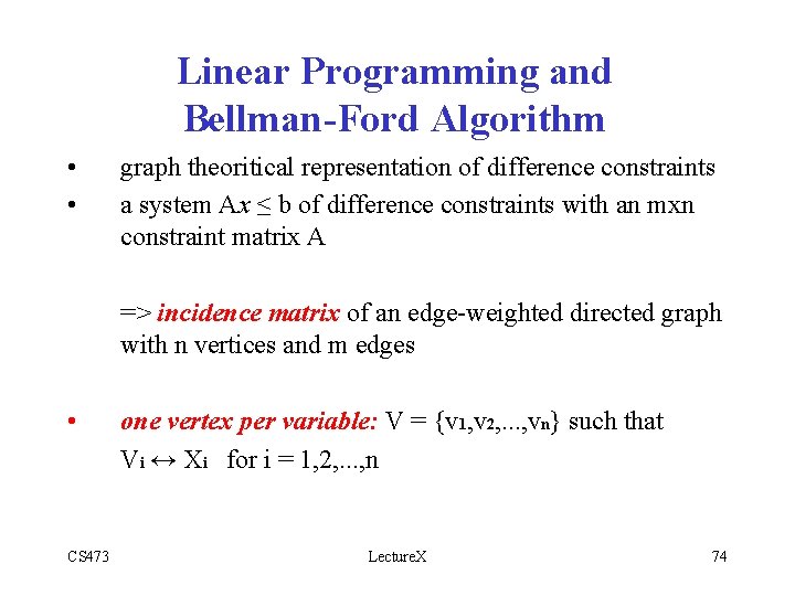
Linear Programming and Bellman-Ford Algorithm • • graph theoritical representation of difference constraints a system Ax ≤ b of difference constraints with an mxn constraint matrix A => incidence matrix of an edge-weighted directed graph with n vertices and m edges • CS 473 one vertex per variable: V = {v 1, v 2, . . . , vn} such that Vi ↔ Xi for i = 1, 2, . . . , n Lecture. X 74

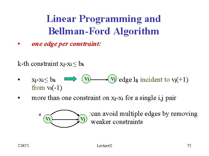
Linear Programming and Bellman-Ford Algorithm • one edge per constraint: k-th constraint xj-xi ≤ bk • • vi vj edge lij incident to vj(+1) xj-xi ≤ bk from vi(-1) more than one constraint on xj-xi for a single i, j pair o CS 473 vi : can avoid multiple edges by removing vj weaker constraints Lecture. X 75

Linear Programming and Bellman-Ford Algorithm • constraint graph for the sample system of difference constraints 1 2 3 4 5 1 1 -1 0 0 0 v 1 b 2 = 1 0 2 1 0 0 0 -1 b 2 = 3 0 1 0 0 -1 b 3 = 1 v 2 v 5 4 -1 0 0 -3 = b 7 5 = b 4 5 -1 0 0 1 0 b 7 = -3 4 = b 5 6 0 0 -1 1 0 v 4 v 3 7 0 0 -1 0 1 b 6 = -1 8 0 0 0 -1 1 CS 473 Lecture. X b 0 -1 1 5 4 -1 -3 -3 76

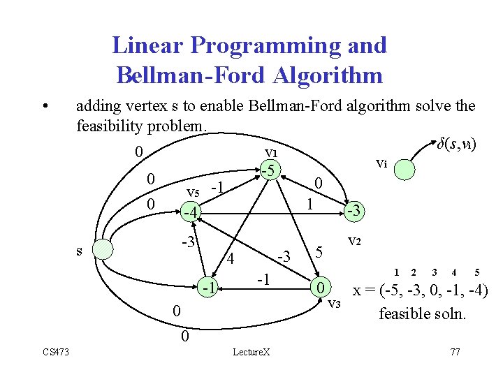
Linear Programming and Bellman-Ford Algorithm • adding vertex s to enable Bellman-Ford algorithm solve the feasibility problem. δ(s, vi) 0 v 1 vi -5 0 0 v 5 -1 0 1 -3 -4 -3 s -3 4 -1 -1 0 v 2 5 1 0 v 3 2 3 4 x = (-5, -3, 0, -1, -4) feasible soln. 0 CS 473 Lecture. X 5 77

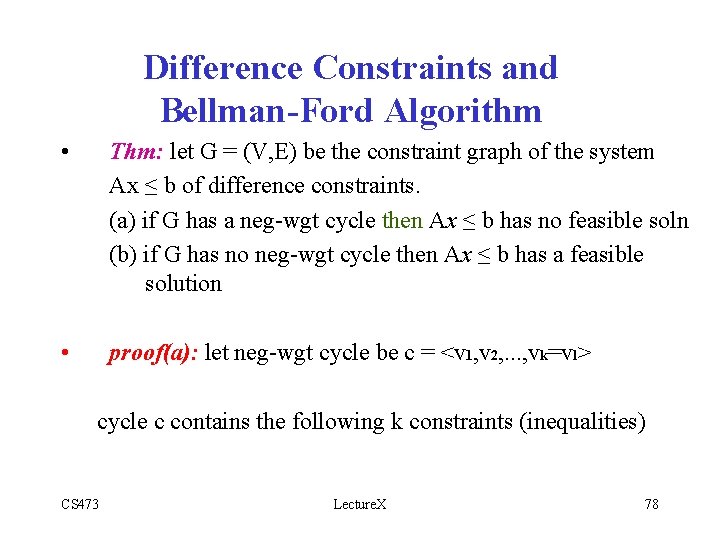
Difference Constraints and Bellman-Ford Algorithm • Thm: let G = (V, E) be the constraint graph of the system Ax ≤ b of difference constraints. (a) if G has a neg-wgt cycle then Ax ≤ b has no feasible soln (b) if G has no neg-wgt cycle then Ax ≤ b has a feasible solution • proof(a): let neg-wgt cycle be c = <v 1, v 2, . . . , vk=vl> cycle c contains the following k constraints (inequalities) CS 473 Lecture. X 78

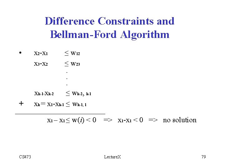
Difference Constraints and Bellman-Ford Algorithm • x 2 -x 1 x 3 -x 2 ≤ w 12 ≤ w 23. . . + xk-1 -xk-2 ≤ wk-2, k-1 xk = x 1 -xk-1 ≤ wk-1, 1 x 1 – x 1 ≤ w(i) < 0 CS 473 => x 1 -x 1 < 0 => no solution Lecture. X 79

Difference Constraints and Bellman-Ford Algorithm • Consider any feasible soln. x for Ax ≤ b o x must satisfy each of these k inequalities o x must also satisfy the inequality that results when we sum them together CS 473 Lecture. X 80

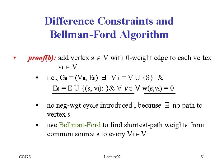
Difference Constraints and Bellman-Ford Algorithm proof(b): add vertex s V with 0 -weight edge to each vertex vi V • i. e. , G 0 = (V 0, E 0) V 0 = V U {S} & E 0 = E U {(s, vi): }& v V w(s, vi) = 0 E • • CS 473 E • no neg-wgt cycle introduced , because no path to vertex s use Bellman-Ford to find shortest-path weights from common source s to every Vi V Lecture. X 81

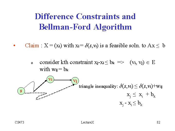
Difference Constraints and Bellman-Ford Algorithm • Claim : X = (xi) with xi = δ(s, vi) is a feasible soln. to Ax ≤ b o consider kth constraint xj-xi ≤ bk => with wij = bk vi s CS 473 vj (vi, vj) E triangle ineaquality: δ(s, vi) ≤ δ(s, vi)+wij xj ≤ xi + bk xj - xi ≤ bk Lecture. X 82

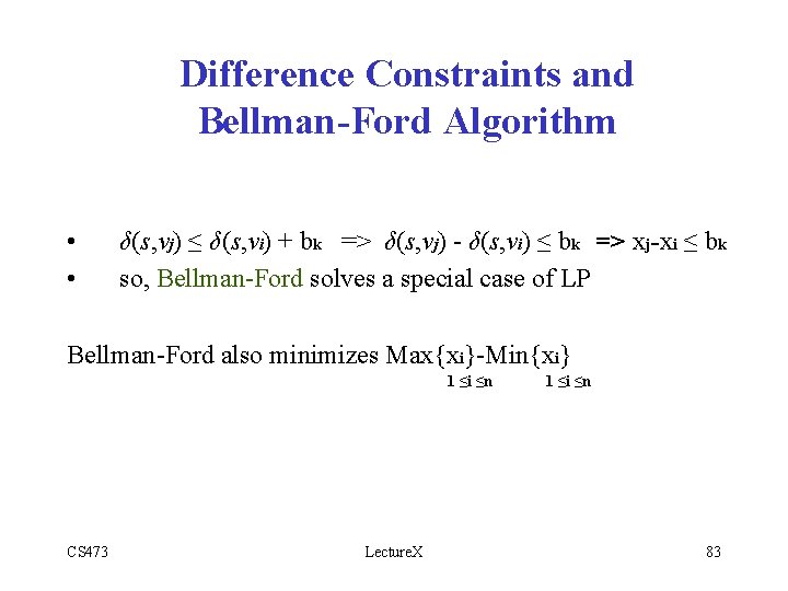
Difference Constraints and Bellman-Ford Algorithm • • δ(s, vj) ≤ δ(s, vi) + bk => δ(s, vj) - δ(s, vi) ≤ bk => xj-xi ≤ bk so, Bellman-Ford solves a special case of LP Bellman-Ford also minimizes Max{xi}-Min{xi} 1 ≤i ≤n CS 473 Lecture. X 1 ≤i ≤n 83