CS 4100 Artificial Intelligence Prof C Hafner Class

CS 4100 Artificial Intelligence Prof. C. Hafner Class Notes Feb 28 and March 13 -15, 2012

Uncertain knowledge/beliefs arise from • Chance (probability) • Incomplete knowledge – Defeasible (“default”) reasoning – Reasoning from ignorance • Ambiguous or conflicting evidence – Evidential reasoning • Vagueness – Fuzzy / open-textured concepts

Examples • Chance – Will your first child be a boy or girl (before conceived) – Will the coin come up heads or tails • Defeasible reasoning: – If I believe Tweety is a bird, then I think he can fly – If I learn Tweety is a penguin then I think he can’t fly • Assuming the normal case unless/until you learn otherwise • Reasoning from ignorance: – I believe the President of the US is alive

Examples (cont. ) • “Evidential reasoning” - how strongly do I believe P based on the evidence? (Confidence levels) – Quantitative [ 0 , 1 ], [ -1 , 1 ] – Qualitative {definite; very likely, neutral, unlikely, very unlikely, definitely not} • Fuzzy concepts: – John is tall – My friend promises to return a book “soon” • Add “degree” to fuzzy assertions (between 0 and 1)

Some problems Using probability, if we know P(A) and P(B) we have methods for calculating P(~A), P(A and B), P(A or B), P(A | B) Using evidential or fuzzy models, these cause problems of consistency: If “John is tall”. 8 and “John is smart”. 6 what can be said about “John is both tall and smart” ? We will mainly focus on probabilistic reasoning models

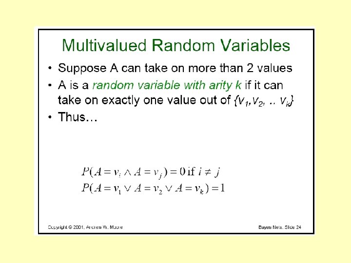
Syntax for probabilistic reasoning • Basic element: random variable • Similar to propositional logic: possible worlds defined by assignment of values to random variables. • Boolean random variables e. g. , Cavity (do I have a cavity? ) • Discrete random variables e. g. , Weather is one of <sunny, rainy, cloudy, snow> • Domain values must be exhaustive and mutually exclusive • Elementary proposition constructed by assignment of a value to a single random variable: e. g. , Weather = sunny, Cavity = false (sometime abbreviated as cavity) • Complex propositions formed from elementary propositions and standard logical connectives e. g. , Weather = sunny Cavity = false

Syntax • Atomic event: A complete specification of the state of the world about which the agent is uncertain • E. g. , if the world consists of only two Boolean variables Cavity and Toothache, then there are 4 distinct atomic events: Cavity = false Toothache = false Cavity = false Toothache = true Cavity = true Toothache = false Cavity = true Toothache = true • Atomic events are mutually exclusive and exhaustive (often called “Outcomes”) • Events in general are sets of atomic events, such as “Cavity = true”

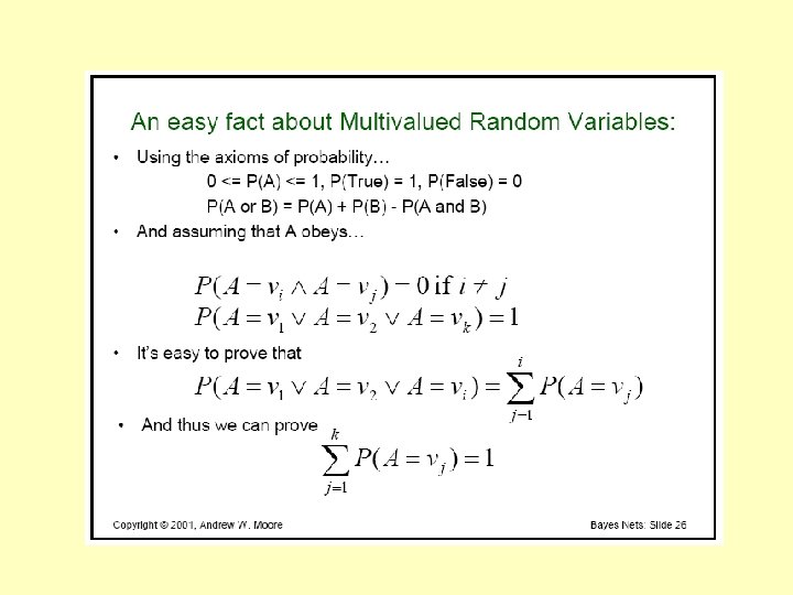
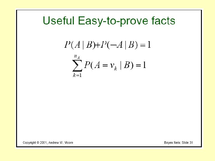
Axioms of probability • For any propositions A, B – 0 ≤ P(A) ≤ 1 – P(true) = 1 and P(false) = 0 – P(A B) = P(A) + P(B) - P(A B)

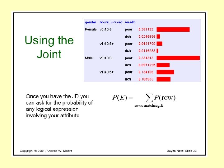
Prior probability • Prior or unconditional probabilities of propositions e. g. , P(Cavity = true) = 0. 1 and P(Weather = sunny) = 0. 72 correspond to belief prior to arrival of any (new) evidence • Probability distribution gives values for all possible assignments: P(Weather) = <0. 72, 0. 1, 0. 08, 0. 1> (sums to 1) • Joint probability distribution for a set of random variables gives the probability of every atomic event on those random variables: P(Weather, Cavity) = a 4 × 2 matrix of values: Weather = Cavity = true Cavity = false sunny rainy cloudy snow 0. 144 0. 02 0. 016 0. 02 0. 576 0. 08 0. 064 0. 08 • Every probability question about a domain can be answered by the joint distribution

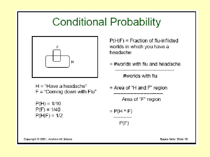
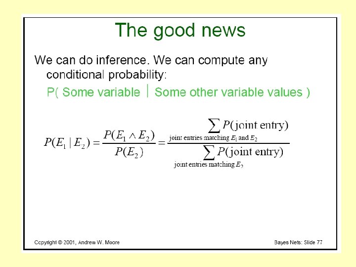
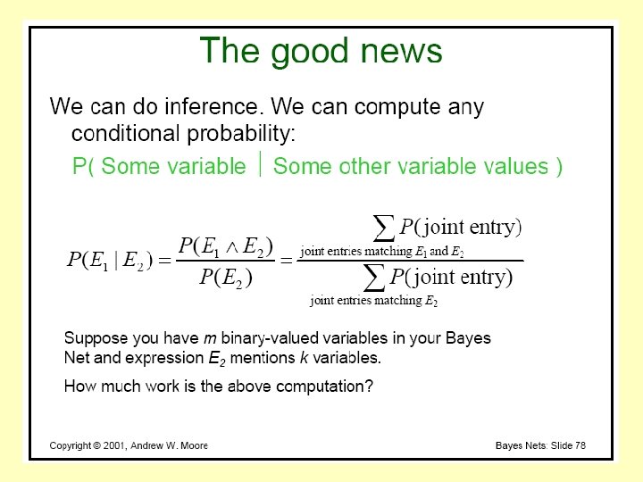
Conditional probability • Conditional or posterior probabilities e. g. , P(cavity | toothache) = 0. 8 i. e. , given that toothache is all I know • (Notation for conditional distributions (use boldface): P(Cavity | Toothache) = 2 -element vector of 2 -element vectors) • If we know more, e. g. , cavity is also given, then we have P(cavity | toothache, cavity) = 1 • New evidence may be irrelevant, allowing simplification, e. g. , cavity does not depend on weather: P(cavity | toothache, sunny) = P(cavity | toothache) = 0. 8 • This kind of inference, sanctioned by domain knowledge, is crucial for probabilistic reasoning in AI. WHY?

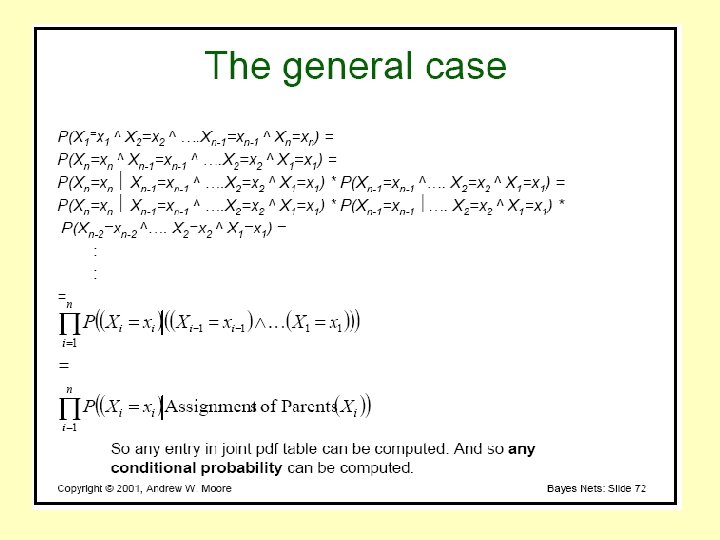
Conditional probability • Definition of conditional probability: P(a | b) = P(a b) / P(b) if P(b) > 0 • Product rule gives an alternative formulation: P(a b) = P(a | b) P(b) = P(b | a) P(a) • A general version holds for whole distributions, e. g. , P(Weather, Cavity) = P(Weather | Cavity) P(Cavity) • (View as a set of 4 × 2 equations, not matrix mult. ) • Chain rule is derived by successive application of product rule: P(X 1, …, Xn) = P(X 1, . . . , Xn-1) P(Xn | X 1, . . . , Xn-1) = P(X 1, . . . , Xn-2) P(Xn-1 | X 1, . . . , Xn-2) P(Xn | X 1, . . . , Xn-1) =… = P(X 1) P(X 2 | X 1) P(X 3 | X 1, X 2). . . P(Xn | X 1, . . . , Xn-1) OR: πi= 1 to n P(Xi | X 1, … , Xi-1)

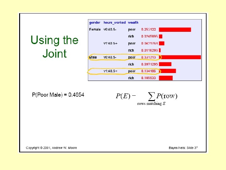
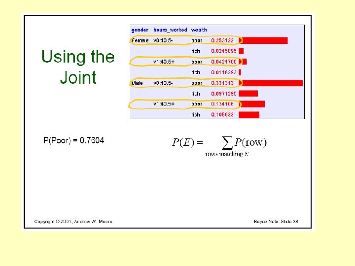
Inference by enumeration • Start with the joint probability distribution: • For any proposition φ, sum the atomic events where it is true: P(φ) = Σω: ω╞φ P(ω)

Inference by enumeration • Start with the joint probability distribution: • For any proposition φ, sum the atomic events where it is true: P(φ) = Σω: ω╞φ P(ω) • P(toothache) = 0. 108 + 0. 012 + 0. 016 + 0. 064 = 0. 2

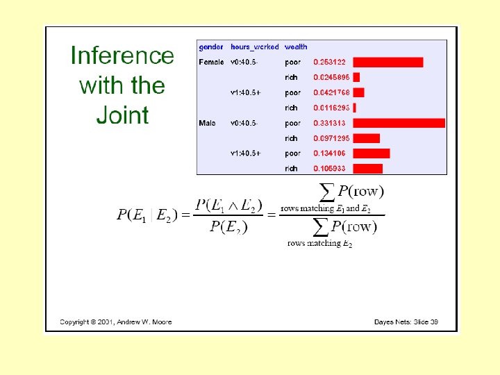
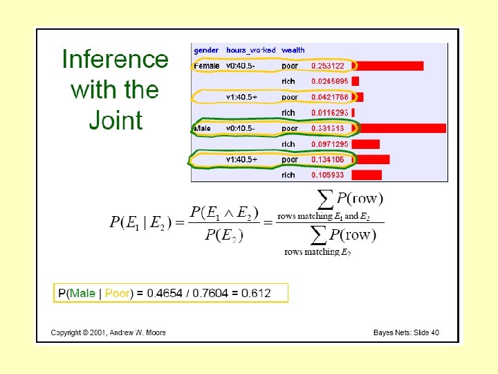
Inference by enumeration • Start with the joint probability distribution: • Can also compute conditional probabilities: P( cavity | toothache) = P( cavity toothache) P(toothache) = 0. 016+0. 064 0. 108 + 0. 012 + 0. 016 + 0. 064 = 0. 4

In class exercise • Given the joint distribution shown on slide and the definition P(a | b) = P(a b) / P(b): – What is P(Cavity = True) ? – What is P(Weather = Sunny) ? – What is P(Cavity = True | Weather = Sunny) • Given the meta-equation: – P(Weather, Cavity) = P(Weather | Cavity) P(Cavity) What are the 8 equations represented here? Weather = Cavity = true Cavity = false sunny rainy cloudy snow 0. 144 0. 02 0. 016 0. 02 0. 576 0. 08 0. 064 0. 08

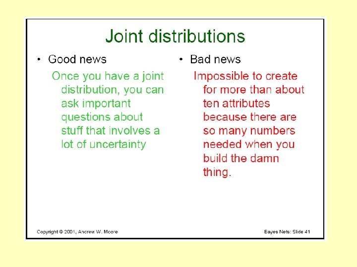
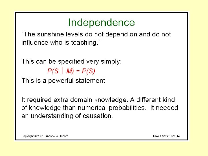
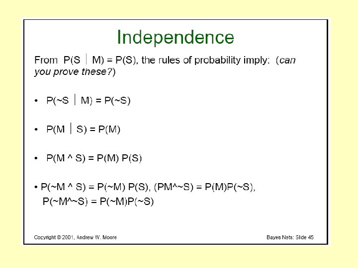
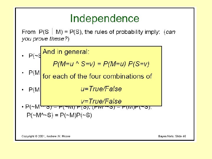
Independence • A and B are independent iff P(A|B) = P(A) or P(B|A) = P(B) or P(A, B) = P(A) P(B) P(Toothache, Catch, Cavity, Weather) = P(Toothache, Catch, Cavity) P(Weather) • 32 entries reduced to 12; for n independent biased coins, O(2 n) →O(n) • Absolute independence powerful but rare • Dentistry is a large field with hundreds of variables, none of which are independent. What to do?

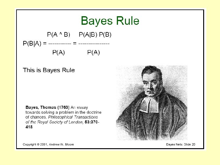
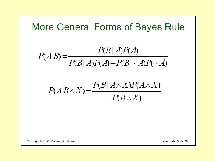
Bayes' Rule • Product rule P(a b) = P(a | b) P(b) = P(b | a) P(a) Bayes' rule: P(a | b) = P(b | a) P(a) / P(b) • or in distribution form P(Y|X) = P(X|Y) P(Y) / P(X) = αP(X|Y) P(Y) • Useful for assessing diagnostic probability from causal probability: – P(Cause|Effect) = P(Effect|Cause) P(Cause) / P(Effect) – E. g. , let M be meningitis, S be stiff neck: P(m|s) = P(s|m) P(m) / P(s) = 0. 8 × 0. 0001 / 0. 1 = 0. 0008 – Note: posterior probability of meningitis still very small!

Example: Expert Systems for Medical Diagnosis • 100 diseases • 20 symptoms • # of parameters needed to calculate P(Di) when a patient provides his/her symptoms • Strategy to reduce the size: assume independence of symptoms • Recalculate number of parameters needed

Bayes' Rule and conditional independence P(Cavity | toothache catch) = αP(toothache catch | Cavity) P(Cavity) = αP(toothache | Cavity) P(catch | Cavity) P(Cavity) • This is an example of a naïve Bayes model: P(Cause, Effect 1, … , Effectn) = P(Cause) πi. P(Effecti|Cause) • Total number of parameters is linear in n

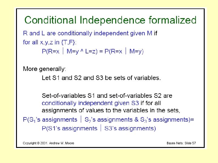
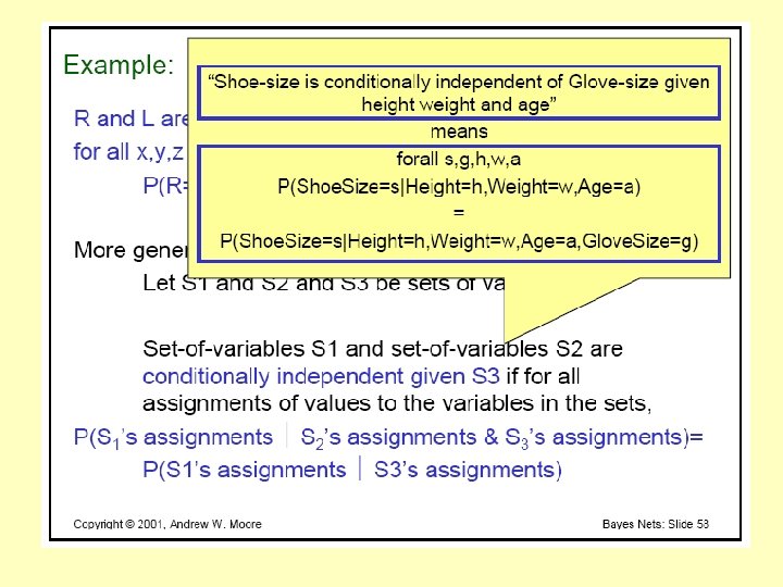
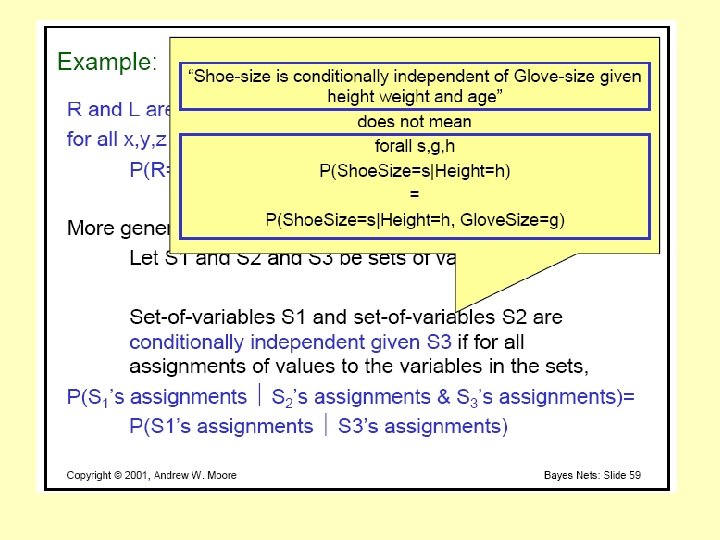
Conditional independence • P(Toothache, Cavity, Catch) has 23 – 1 = 7 independent entries • If I have a cavity, the probability that the probe catches in it doesn't depend on whether I have a toothache: (1) P(catch | toothache, cavity) = P(catch | cavity) • The same independence holds if I haven't got a cavity: (2) P(catch | toothache, cavity) = P(catch | cavity) • Catch is conditionally independent of Toothache given Cavity: P(Catch | Toothache, Cavity) = P(Catch | Cavity) • Equivalent statements: P(Toothache | Catch, Cavity) = P(Toothache | Cavity) P(Toothache, Catch | Cavity) = P(Toothache | Cavity) P(Catch | Cavity)

Conditional independence contd. • Write out full joint distribution using chain rule: P(Toothache, Catch, Cavity) = P(Toothache | Catch, Cavity) P(Catch | Cavity) P(Cavity) = P(Toothache | Cavity) P(Catch | Cavity) P(Cavity) I. e. , 2 + 1 = 5 independent numbers • In most cases, the use of conditional independence reduces the size of the representation of the joint distribution from exponential in n to linear in n. • Conditional independence is our most basic and robust form of knowledge about uncertain environments.

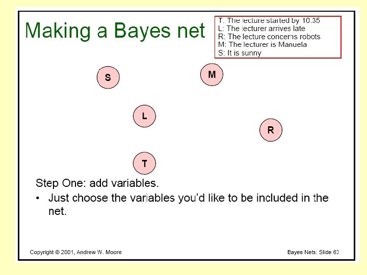
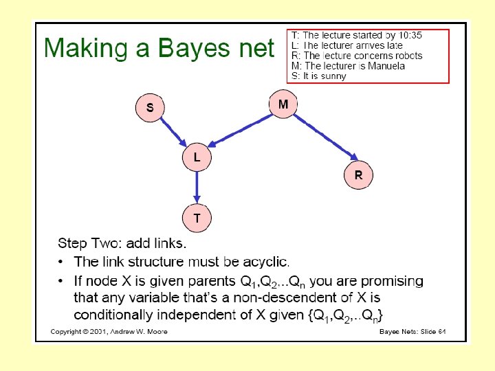
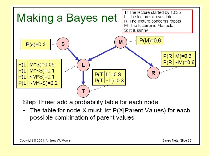
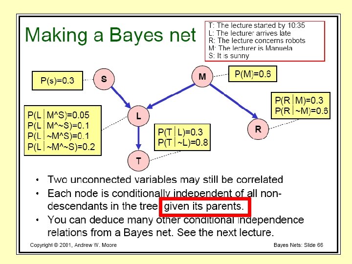
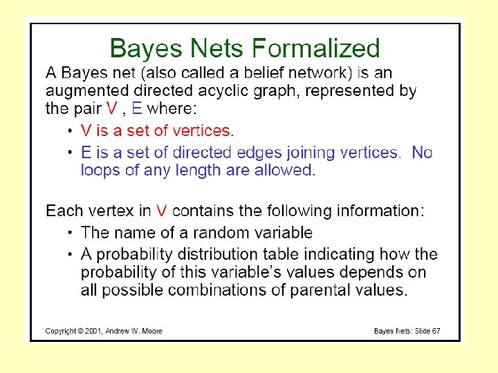
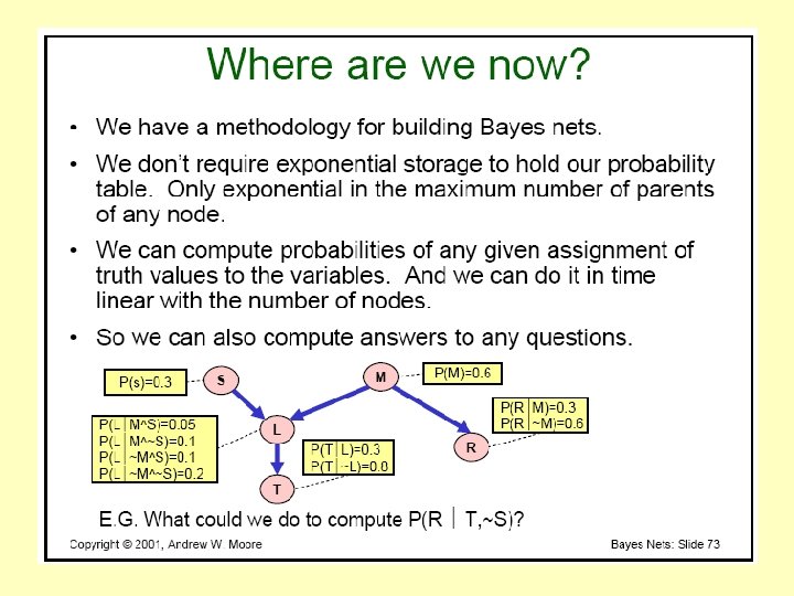
Bayesian networks • A simple, graphical notation for conditional independence assertions and hence for compact specification of full joint distributions • Syntax: – a set of nodes, one per variable – a directed, acyclic graph (link ≈ "directly influences") – a conditional distribution for each node given its parents: P (Xi | Parents (Xi)) • In the simplest case, conditional distribution represented as a conditional probability table (CPT) giving the distribution over Xi for each combination of parent values

Probabilities/Bayesian Inference Nets • Thanks to Andrew Moore from CMU for some great slides. (used with permission)

Review: Conditional probabilities and JPD (joint distribution) Extend to P(A ^ B ^ C ^ …) = ?

Chain rule follows from this definition • Product rule P(a b) = P(a | b) P(b) = P(b | a) P(a) • Chain rule is derived by successive application of product rule: P(X 1, …, Xn) can also be written P(X 1 ^. . . ^ Xn) = P([Xn ^ [X 1 , . . . Xn-1]) = P(X 1, . . . Xn-1) P(Xn | X 1, . . . , Xn-1) = P(X 1, . . . , Xn-2) P(Xn-1 | X 1, . . . , Xn-2) P(Xn | X 1, . . . , Xn-1) =… = P(X 1) P(X 2 | X 1) P(X 3 | X 1, X 2). . . P(Xn | X 1, . . . , Xn-1)

Conditional Prob. example

Example Likes Football Dislikes Neutral Male . 25 . 15 Female . 1 . 3 . 1 In-class exercise: Calculate: P(Likes Football | Male ) P( ~ Likes Football | Female)

Review the Joint Distribution (JPD)

What assumption can we make ?

Test your understanding: Fill in the table

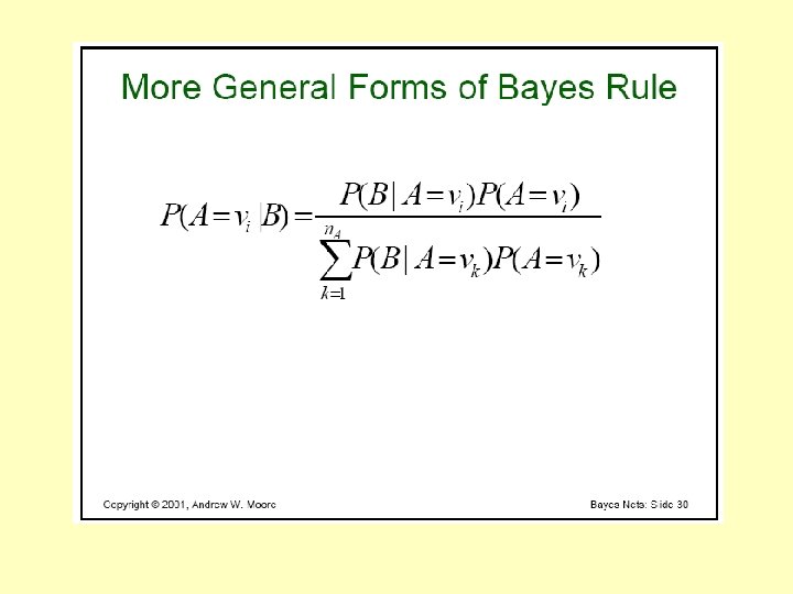
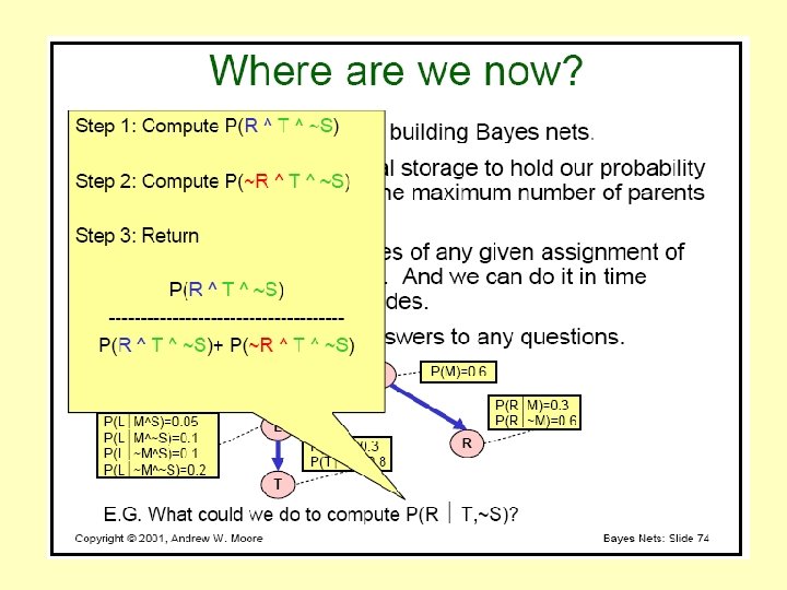
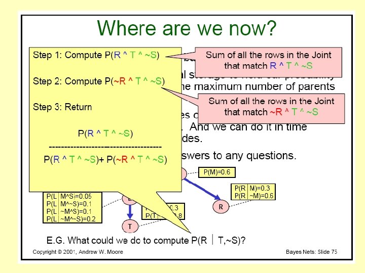
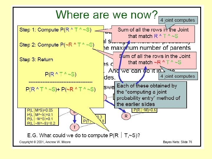
Structure for CP-based AI Models Given a set of RV’s X, typically, we are interested in the posterior joint distribution of the query variables Y given specific values e for the evidence variables E Let the hidden variables be H = X - Y – E Then the required calculation of P(Y | E) is done by summing out the hidden variables: P( Y | E = e) = αP(Y ^ E = e) or αΣh. P(Y ^ E= e ^ H = h) Note: what is α ? Given the definition: P(a | b) = P(a b) / P(b) α is the denominator 1/P(E=e) can be calculated from the joint distribution as: Σh. P(E= e ^ H = h)

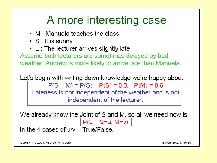
Example (medical diagnosis) Causal model: D I S (Y H E) Cancer anemia fatigue Kidney disease anemia fatigue P(Y=cancer | E=fatigue) = α [ P(Y=cancer ^ E=fatigue ^ anemia) + P(Y=cancer ^ E=fatigue ^ ~anemia) ] α = 1/P(E = fatigue) or 1/[P(E=fatigue ^ anemia) + P(E=fatigue ^ ~anemia) ]

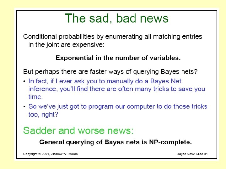
Analysis P(Y | E = e) = αP(Y ^ E = e) = αΣh. P(Y ^ E= e ^ H = h) [repeated] • The terms in the summation are joint entries because Y, E and H together exhaust the set of random variables • Obvious problems: 1. Time and space complexity O(dn) where d is the largest arity 2. How to find the numbers to solve real problems? (A solution to 1. : assume independence !!)

What is Independence ? ? • A and B are independent iff P(A|B) = P(A) or P(B|A) = P(B) or P(A, B) = P(A) P(B) P(Toothache, Catch, Cavity, Weather) JD entries are 2 x 2 x 2 x 4 = P(Toothache, Catch, Cavity) P(Weather) entries are 2 x 2 x 2 + 4 • 32 entries reduced to 12 • In general, total independence assumption reduces exponential to linear complexity

What is Independence ? ? • A and B are independent iff P(A|B) = P(A) or P(B|A) = P(B) or P(A, B) = P(A) P(B) • Toss 10 coins, different OUTCOMES are 2^10 = 2048 • Biased coins whose behavior is independent of each other: O(2 n) →O(n) = can compute P(all outcomes) with 10 values • All coins have the same bias (includes the case of fair coins) ? ? How many values are needed ? Test your understanding: • Consider a “ 3 sided coin” (or die). How many entries needed to show the probabilities of all outcomes? • If you toss 10 of those and: • All have the same bias? • Bias unknown, but independence is assumed? • Bias unknown, no independence assumed?

Example: Expert Systems for Medical Diagnosis • 10 diseases • 20 symptoms • # of parameters needed to calculate P(D | S) for all combinations using a JPD • Strategy to reduce the size of the model: assume mutual independence of symptoms and diseases Recalculate number of parameters needed • Absolute independence powerful but rare • Medicine is a large field with hundreds of variables, many of which are not independent. What to do?

Problem 2: We still need to find the numbers Assuming independence, doctors may be able to estimate: P(symptom | disease) for each S/D pair (causal reasoning) While what we need to know s/he may not be able to estimate as easily: P(disease | symptom) Thus, the importance of Bayes rule in probabilistic AI

Bayes' Rule • Product rule P(a b) = P(a | b) P(b) = P(b | a) P(a) Bayes' rule: P(a | b) = P(b | a) P(a) / P(b) • or in distribution form P(Y|X) = P(X|Y) P(Y) / P(X) = αP(X|Y) P(Y) • Useful for assessing diagnostic probability from causal probability: P(Cause|Effect) = P(Effect|Cause) P(Cause) / P(Effect) P(Disease|Symptom) = P(Symptom|Diease) P(Symptom) / (Disease) – E. g. , let M be meningitis, S be stiff neck: P(m|s) = P(s|m) P(m) / P(s) = 0. 8 × 0. 0001 / 0. 1 = 0. 0008 – Note: posterior probability of meningitis still very small!

Bayes' Rule and conditional independence P(Cavity | toothache catch) = αP(toothache catch | Cavity) P(Cavity) = αP(toothache | Cavity) P(catch | Cavity) P(Cavity) • We say: “toothache and catch are independent, given cavity”. This is an example of a naïve Bayes model. We will study this later as our simplest machine learning application P(Cause, Effect 1, … , Effectn) = P(Cause) πi. P(Effecti|Cause) • Total number of parameters is linear in n (number of symptoms). This is our first Bayesian inference net.

Conditional independence • P(Toothache, Cavity, Catch) has 23 – 1 = 7 independent entries • If I have a cavity, the probability that the probe catches in it doesn't depend on whether I have a toothache: (1) P(catch | toothache, cavity) = P(catch | cavity) • The same independence holds if I haven't got a cavity: (2) P(catch | toothache, cavity) = P(catch | cavity) • Catch is conditionally independent of Toothache given Cavity: P(Catch | Toothache, Cavity) = P(Catch | Cavity) • Equivalent statements (from original definitions of independence): P(Toothache | Catch, Cavity) = P(Toothache | Cavity) P(Toothache, Catch | Cavity) = P(Toothache | Cavity) P(Catch | Cavity)

Conditional independence contd. • Write out full joint distribution using chain rule: P(Toothache, Catch, Cavity) = P(Toothache | Catch, Cavity) P(Catch | Cavity) P(Cavity) = P(Toothache | Cavity) P(Catch | Cavity) P(Cavity) I. e. , 2 + 1 = 5 independent numbers • In most cases, the use of conditional independence reduces the size of the representation of the joint distribution from exponential in n to linear in n. • Conditional independence is our most basic and robust form of knowledge about uncertain environments.

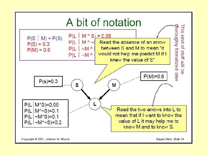
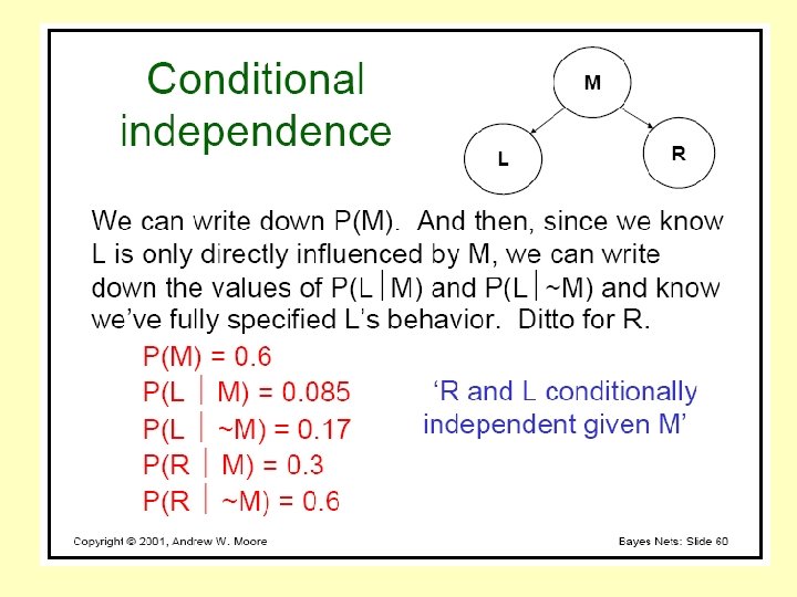
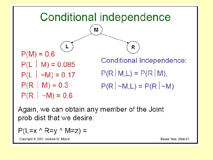
Remember this examples

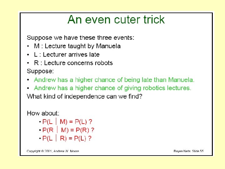
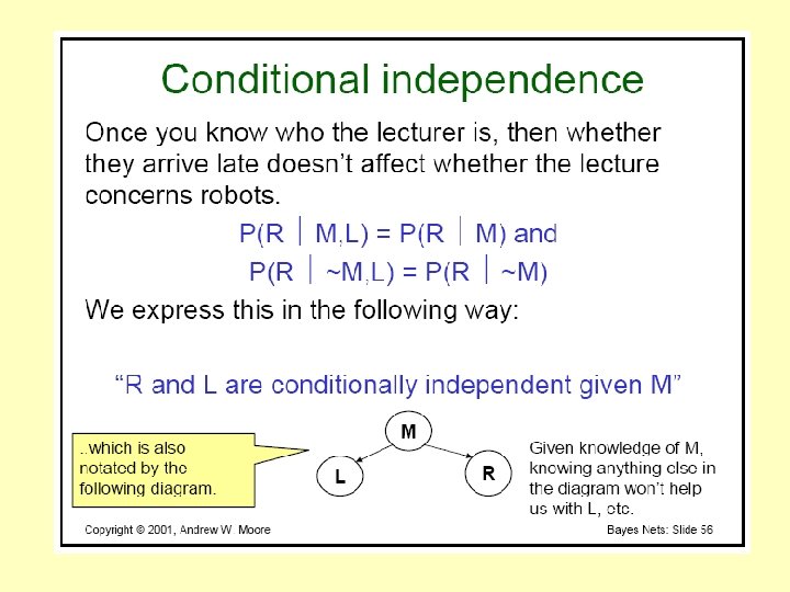
Example of conditional independence

Test your understanding of the Chain Rule

This is our second Bayesian inference net

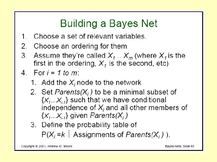
How to construct a Bayes Net

Test your understanding: design a Bayes net with plausible numbers

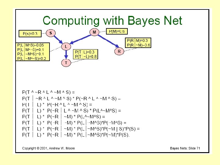
Calculating using Bayes’ Nets