CS 4100 Artificial Intelligence Prof C Hafner Class

CS 4100 Artificial Intelligence Prof. C. Hafner Class Notes March 27, 2012

Term Project Presentations • Homework 6 is due Tuesday in class (hard copy) • We need 4 teams to volunteer to make presentations on April 12 !! • The other 5 teams will make presentations on April 17 (last day) • Each presentation will be strictly limited to 15 minutes, with 3 minutes for discussion/questions. • Make sure your slides/demos load immediately – we do not have time to wait for Google Docs exploration.

Supervised Learning (cont. ) • Decision Tree Learning (actually, classification learning) – return for further discussion • We also consider techniques for evaluating supervised learning systems • Perceptrons/Neural Nets • Naïve Bayes Classifiers • April 3, 5, 10: finish ML, introduce NLP • http: //www. cis. temple. edu/~giorgio/cis 587/readings /id 3 -c 45. html#1.

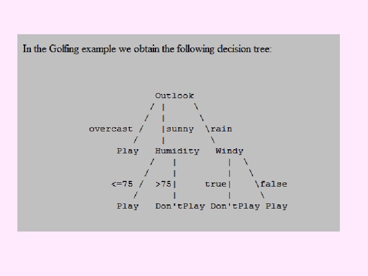
ID 3 and C 4. 5 Golfing Example: Attributes Decision: Play or Don’t Play

ID 3 and C 4. 5 Golfing Example: Training Data Decision: Play or Don’t Play

Stock Market Example

Table of Entropy values • http: //usl. sis. pitt. edu/trurl/log-table. html

Review the Algorithm • In the case of our golfing example, for the attribute Outlook we have • Info(Outlook, T) = 5/14*I(2/5, 3/5) + 4/14*I(4/4, 0) + 5/14*I(3/5, 2/5) = 0. 694 Consider the quantity Gain(X, T) defined as • Gain(X, T) = Info(T) - Info(X, T) This represents the difference between the information needed to identify an element of T and the information needed to identify an element of T after the value of attribute X has been obtained, that is, this is the gain in information due to attribute X. • In our golfing example, for the Outlook attribute the gain is: • Gain(Outlook, T) = Info(T) - Info(Outlook, T) = 0. 94 - 0. 694 = 0. 246. If we instead consider the attribute Windy, we find that Info(Windy, T) is 0. 892 and Gain(Windy, T) is 0. 048. Thus Outlook offers a greater informational gain than Windy.

C 4. 5 Extension Example 1 Notice that in this example two of the attributes have continuous ranges, Temperature and Humidity. ID 3 does not directly deal with such cases. We can deal with the case of attributes with continuous ranges as follows: Say that attribute Ci has a continuous range. We examine the values for this attribute in the training set. Say they are, in increasing order, A 1, A 2, . . , Am. Then for each value Aj, j=1, 2, . . m, we partition the records into those that have Ci values up to and including Aj, and those that have values greater than Aj. For each of these partitions we compute the gain, or gain ratio, and choose the partition that maximizes the gain. This makes Ci a Boolean (or binary) attribute. In our Golfing example, for humidity, if T is the training set, we determine the information for each partition and find the best partition at 75. Then the range for this attribute becomes {<=75, >75}. Notice that this method involves a substantial number of computations.

C 4. 5 Extension Example 2

ID 3 and C 4. 5 • ID 3 algorithm (we learned last time) is important not because it summarizes what we know, i. e. the training set, but because we hope it will classify correctly new cases. Thus when building classification models one should have both training data to build the model and test data to verify how well it actually works. • C 4. 5 is an extension of ID 3 that accounts for unavailable values, continuous attribute value ranges, pruning of decision trees, rule derivation, and so on.

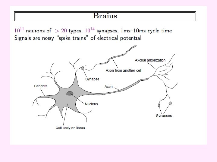
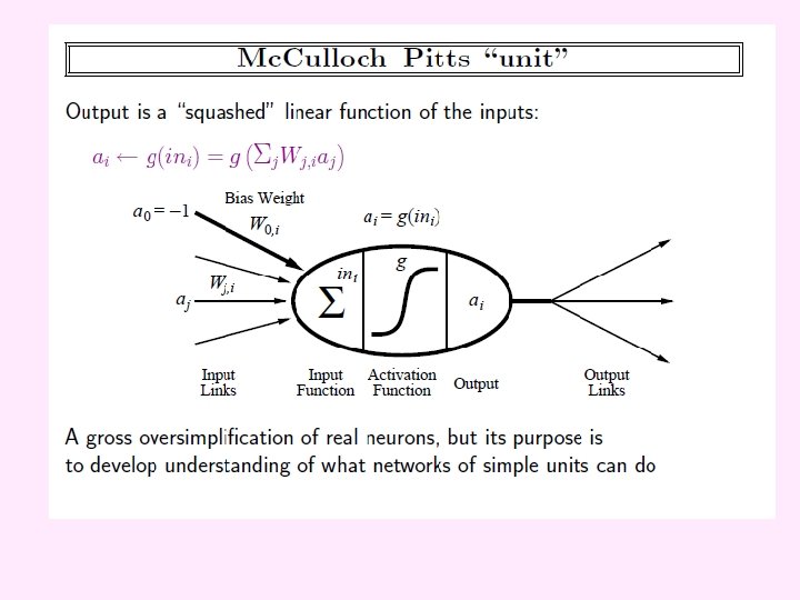
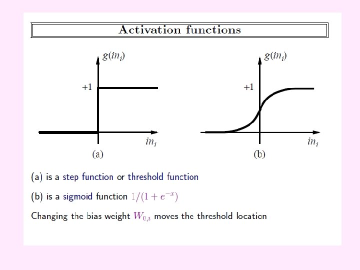
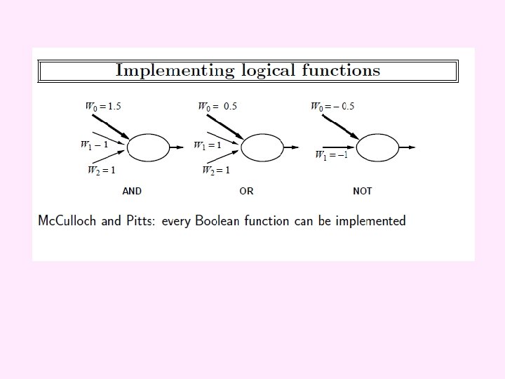
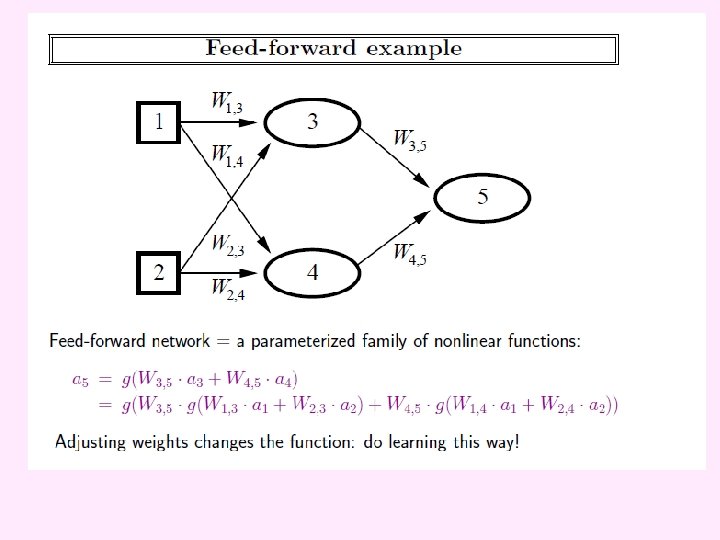
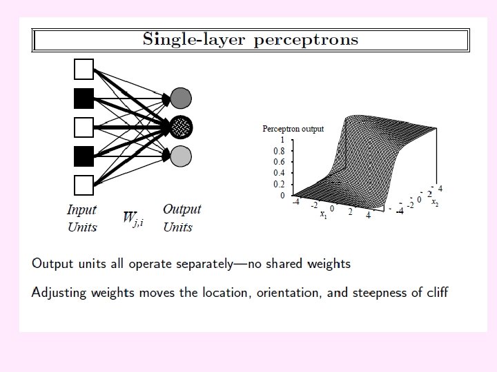
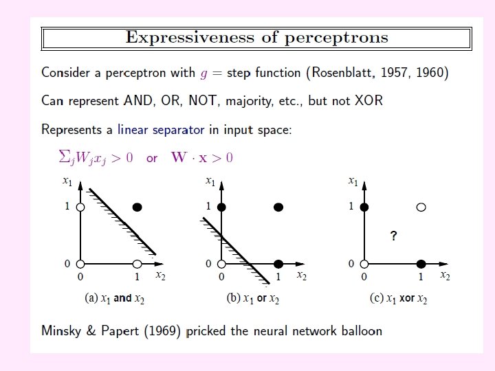
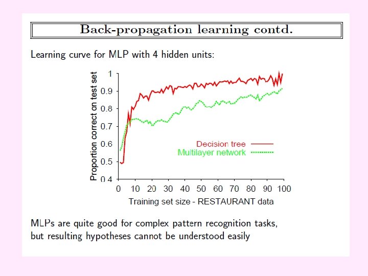
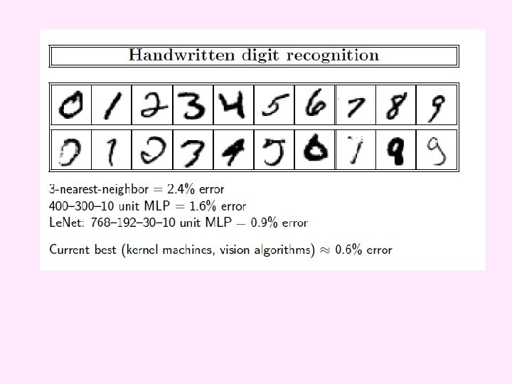
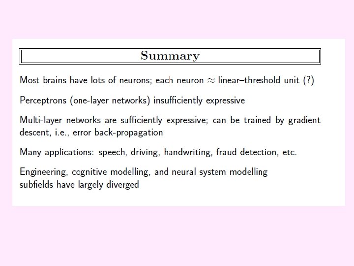
Perceptrons and Neural Networks: Another Supervised Learning Approach

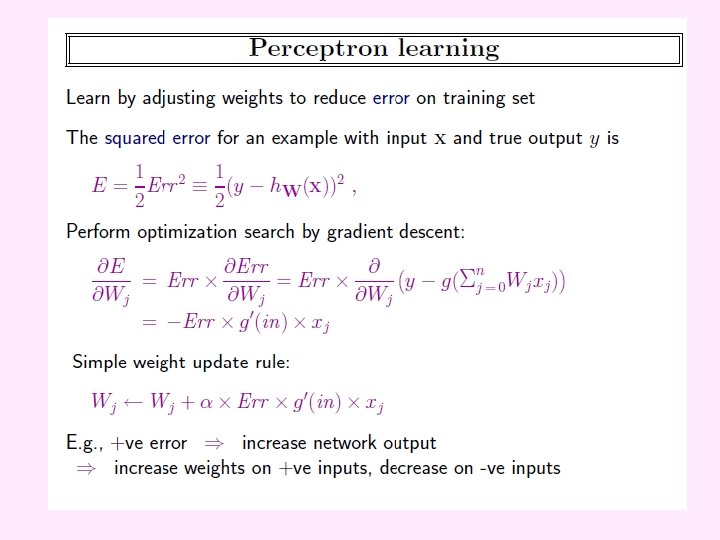
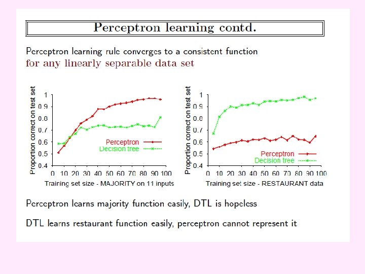
Perceptron Learning (Supervised) • • Assign random weights (or set all to 0) Cycle through input data until change < target Let α be the “learning coefficient” For each input: – If perceptron gives correct answer, do nothing – If perceptron says yes when answer should be no, decrease the weights on all units that “fired” by α – If perceptron says no when answer should be yes, increase the weights on all units that “fired” by α

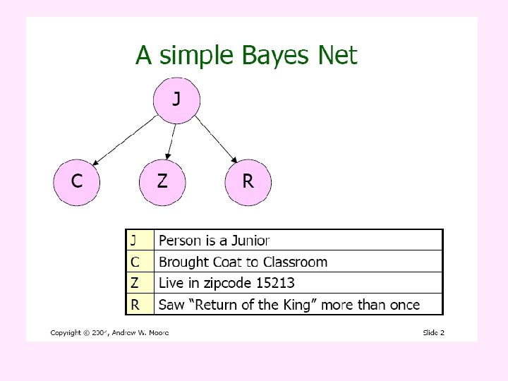
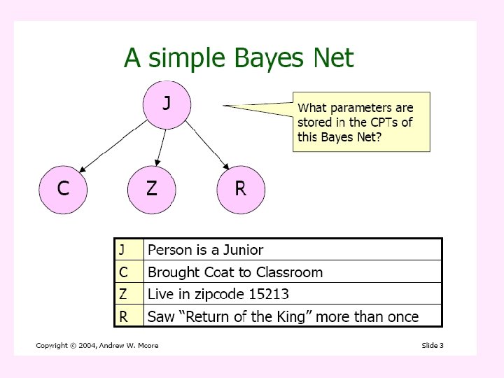
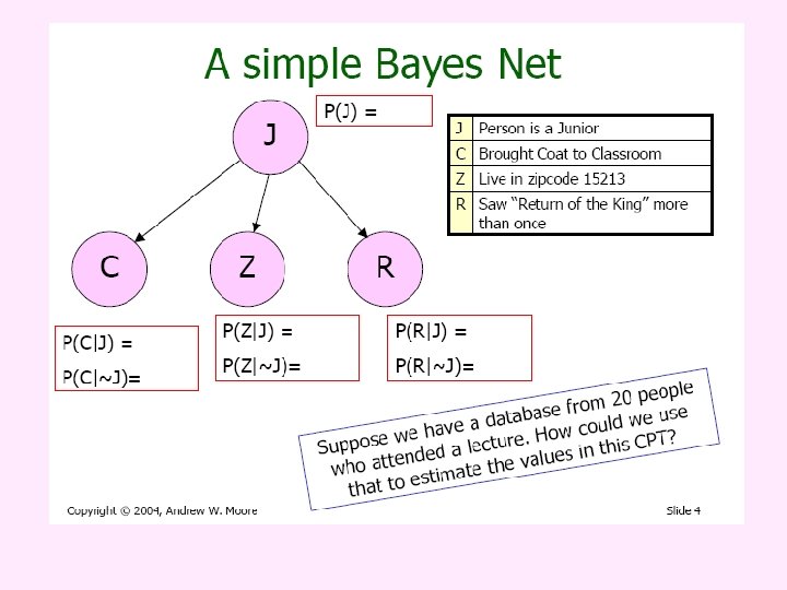
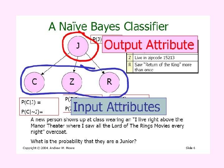
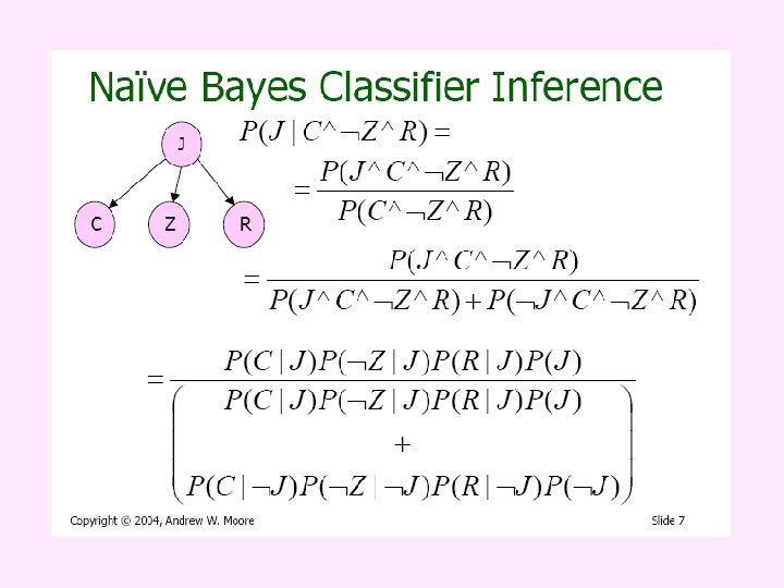
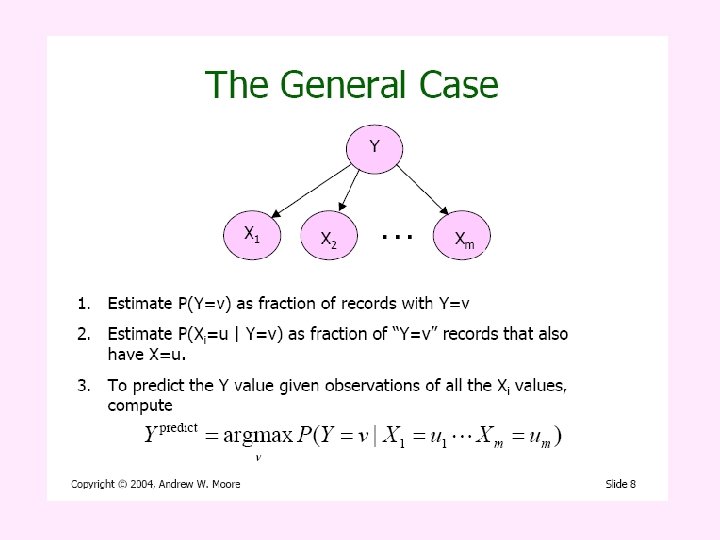
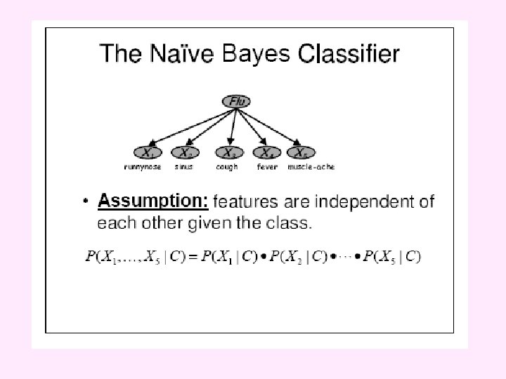
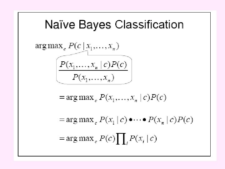
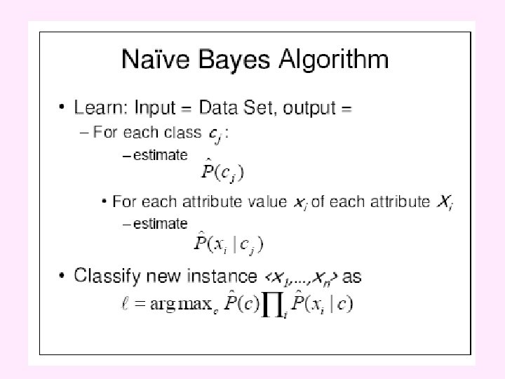
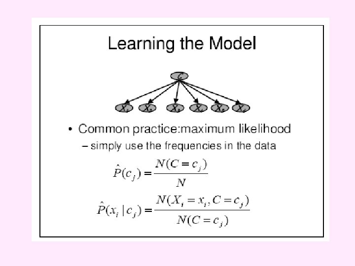
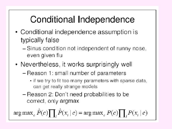
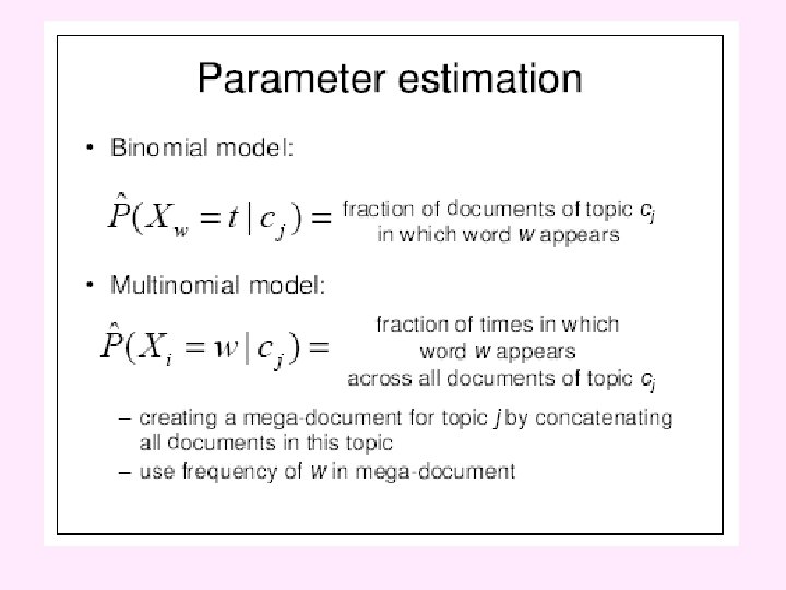
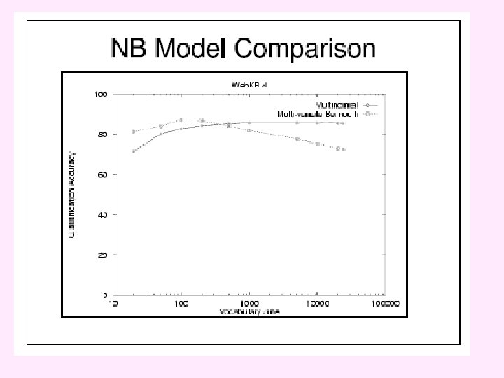
Naive Bayes Classifiers: Our next example of machine learning • A supervised learning method • Making independence assumption, we can explore a simple subset of Bayesian nets, such that: • It is easy to estimate the CPT’s from sample data • Uses a technique called “maximum likelihood estimation” – Given a set of correctly classified representative examples – Q: What estimates of conditional probabilities maximize the likelihood of the data that was observed? – A: The estimates that reflect the sample proportions

# Juniors were Juniors and # Juniors were Non-Juniors # Non-Juniors

Naive Bayes Classifier with multi-valued variables Major: Science, Arts, Social Science Student characteristics: Gender (M, F), Race/Ethnicity (W, B, H, A) International (T/F) What do the conditional probability tables look like? ?

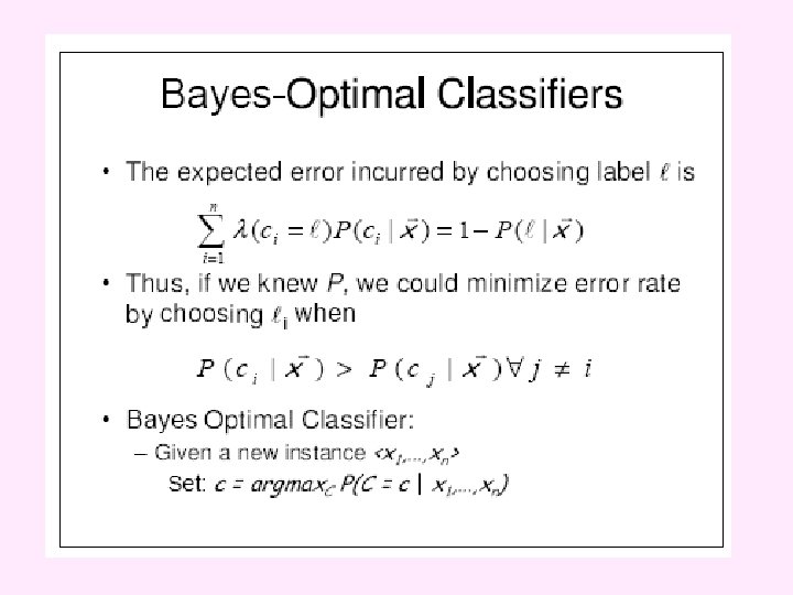
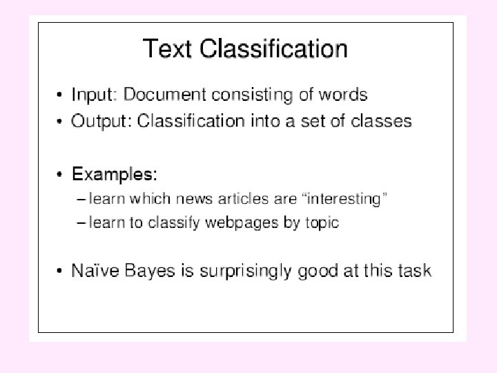
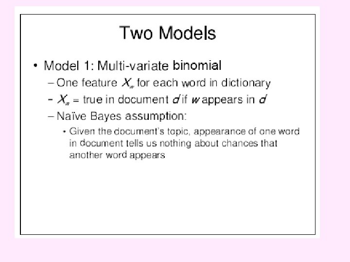
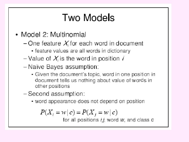
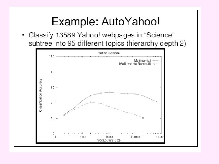
Theoretical Foundation and Application to Text Classification - thanks Prof. Daphne Koller at Stanford