Introduction to Artificial Intelligence Unit 7 A Learning

Introduction to Artificial Intelligence – Unit 7 A Learning Course 67842 The Hebrew University of Jerusalem School of Engineering and Computer Science Academic Year: 2011/2012 Instructor: Jeff Rosenschein (Chapter 18, “Artificial Intelligence: A Modern Approach”)

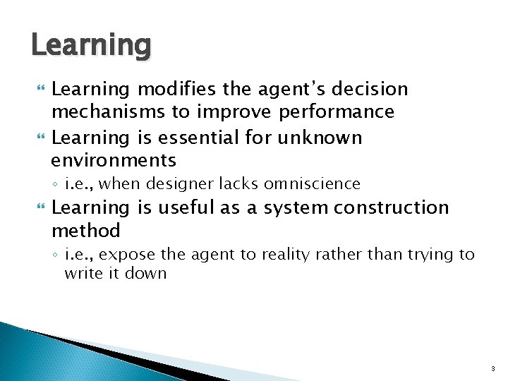
Outline Learning agents Inductive learning Decision tree learning 2

Learning modifies the agent’s decision mechanisms to improve performance Learning is essential for unknown environments ◦ i. e. , when designer lacks omniscience Learning is useful as a system construction method ◦ i. e. , expose the agent to reality rather than trying to write it down 3

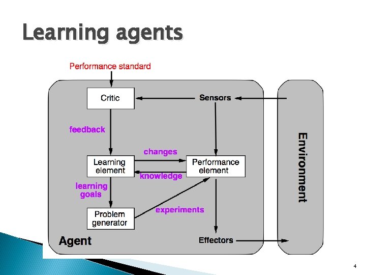
Learning agents 4

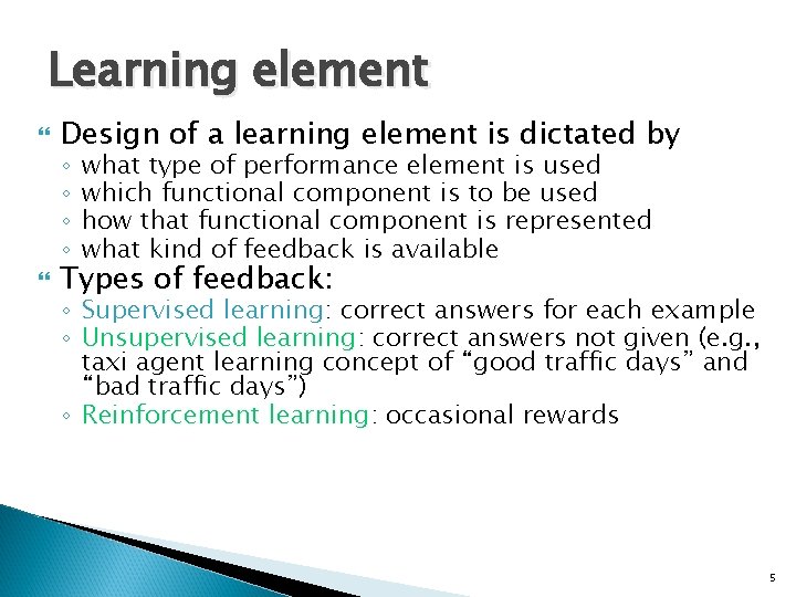
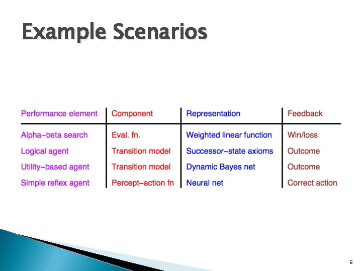
Learning element Design of a learning element is dictated by Types of feedback: ◦ ◦ what type of performance element is used which functional component is to be used how that functional component is represented what kind of feedback is available ◦ Supervised learning: correct answers for each example ◦ Unsupervised learning: correct answers not given (e. g. , taxi agent learning concept of “good traffic days” and “bad traffic days”) ◦ Reinforcement learning: occasional rewards 5

Example Scenarios 6

Aibo Robots Learning to Walk Faster http: //www. cs. utexas. edu/users/Austin. Villa/ ? p=research/learned_walk Aibo Learning Movies 7

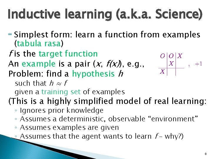
Inductive learning (a. k. a. Science) Simplest form: learn a function from examples (tabula rasa) f is the target function An example is a pair (x, f(x)), e. g. , Problem: find a hypothesis h such that h ≈ f given a training set of examples (This is a highly simplified model of real learning: ◦ ◦ Ignores prior knowledge Assumes a deterministic, observable “environment” Assumes examples are given Assumes that the agent wants to learn f – why? ) 8

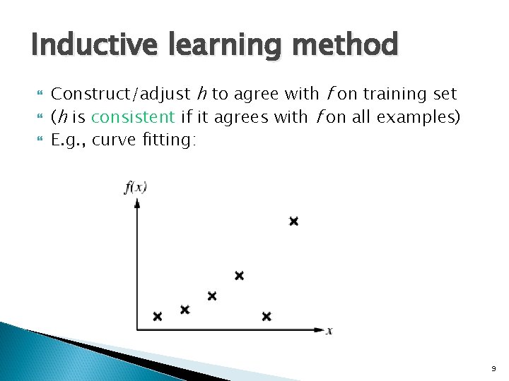
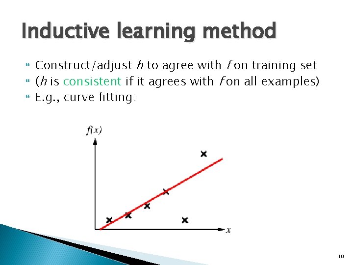
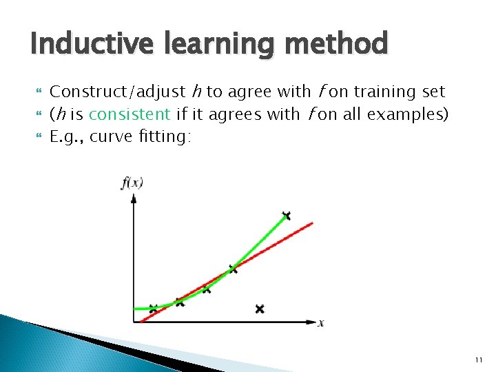
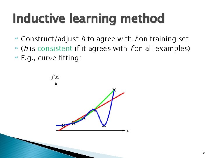
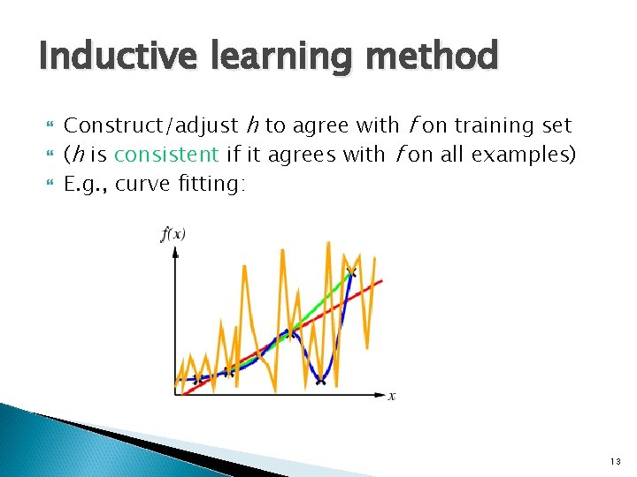
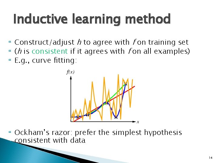
Inductive learning method Construct/adjust h to agree with f on training set (h is consistent if it agrees with f on all examples) E. g. , curve fitting: 9

Inductive learning method Construct/adjust h to agree with f on training set (h is consistent if it agrees with f on all examples) E. g. , curve fitting: 10

Inductive learning method Construct/adjust h to agree with f on training set (h is consistent if it agrees with f on all examples) E. g. , curve fitting: 11

Inductive learning method Construct/adjust h to agree with f on training set (h is consistent if it agrees with f on all examples) E. g. , curve fitting: 12

Inductive learning method Construct/adjust h to agree with f on training set (h is consistent if it agrees with f on all examples) E. g. , curve fitting: 13

Inductive learning method Construct/adjust h to agree with f on training set (h is consistent if it agrees with f on all examples) E. g. , curve fitting: Ockham’s razor: prefer the simplest hypothesis consistent with data 14

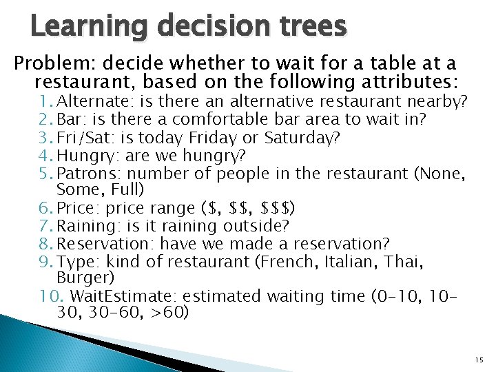
Learning decision trees Problem: decide whether to wait for a table at a restaurant, based on the following attributes: 1. Alternate: is there an alternative restaurant nearby? 2. Bar: is there a comfortable bar area to wait in? 3. Fri/Sat: is today Friday or Saturday? 4. Hungry: are we hungry? 5. Patrons: number of people in the restaurant (None, Some, Full) 6. Price: price range ($, $$$) 7. Raining: is it raining outside? 8. Reservation: have we made a reservation? 9. Type: kind of restaurant (French, Italian, Thai, Burger) 10. Wait. Estimate: estimated waiting time (0 -10, 1030, 30 -60, >60) 15

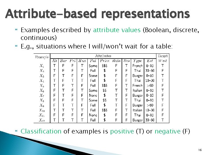
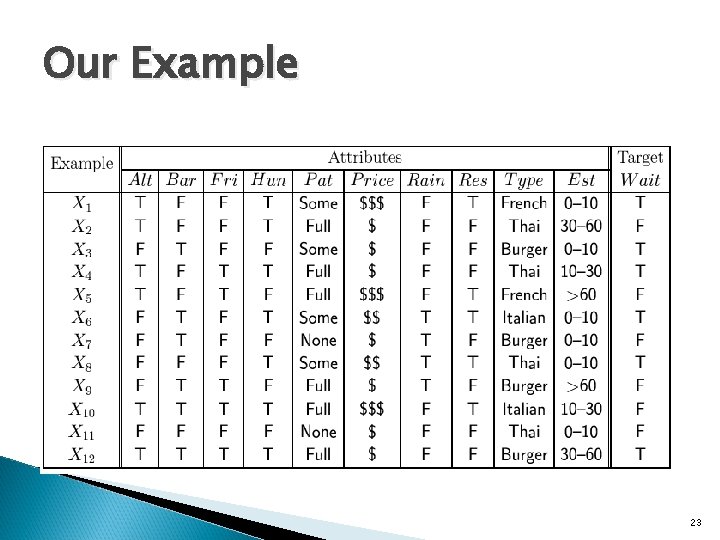
Attribute-based representations Examples described by attribute values (Boolean, discrete, continuous) E. g. , situations where I will/won’t wait for a table: Classification of examples is positive (T) or negative (F) 16

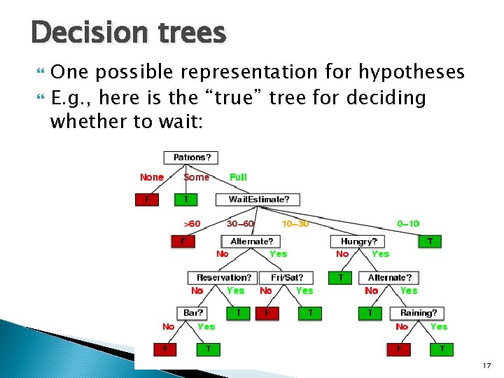
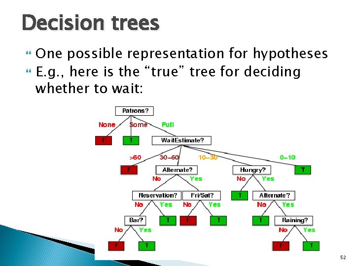
Decision trees One possible representation for hypotheses E. g. , here is the “true” tree for deciding whether to wait: 17

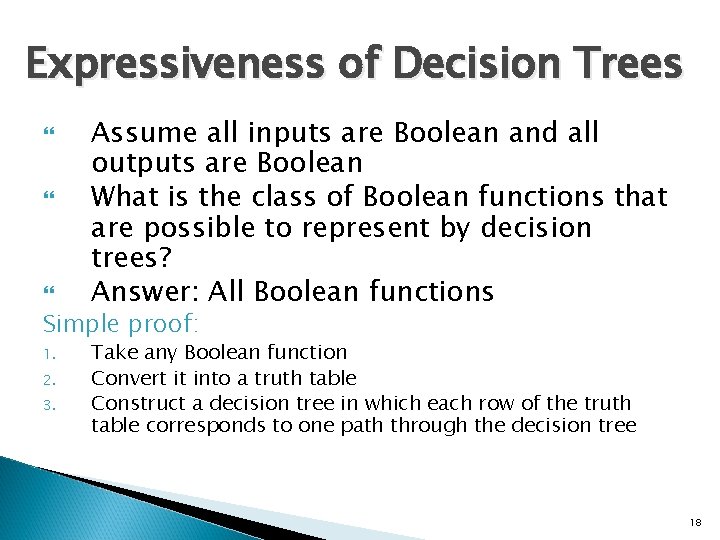
Expressiveness of Decision Trees Assume all inputs are Boolean and all outputs are Boolean What is the class of Boolean functions that are possible to represent by decision trees? Answer: All Boolean functions Simple proof: 1. 2. 3. Take any Boolean function Convert it into a truth table Construct a decision tree in which each row of the truth table corresponds to one path through the decision tree 18

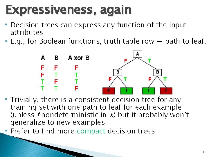
Expressiveness, again Decision trees can express any function of the input attributes E. g. , for Boolean functions, truth table row → path to leaf: Trivially, there is a consistent decision tree for any training set with one path to leaf for each example (unless f nondeterministic in x) but it probably won’t generalize to new examples Prefer to find more compact decision trees 19

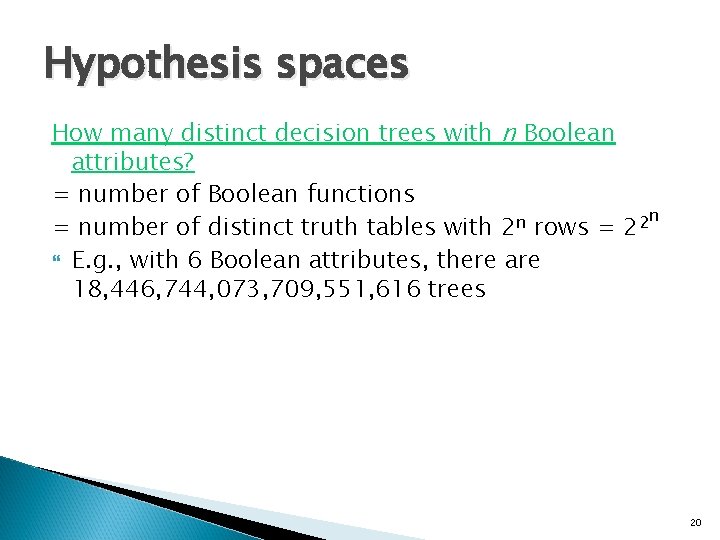
Hypothesis spaces How many distinct decision trees with n Boolean attributes? = number of Boolean functions n = number of distinct truth tables with 2 n rows = 22 E. g. , with 6 Boolean attributes, there are 18, 446, 744, 073, 709, 551, 616 trees 20

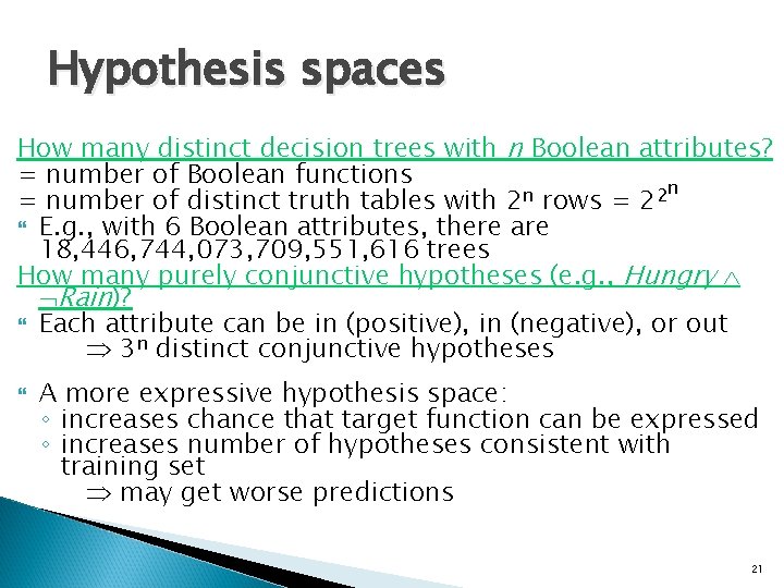
Hypothesis spaces How many distinct decision trees with n Boolean attributes? = number of Boolean functions n n 2 = number of distinct truth tables with 2 rows = 2 E. g. , with 6 Boolean attributes, there are 18, 446, 744, 073, 709, 551, 616 trees How many purely conjunctive hypotheses (e. g. , Hungry Rain)? Each attribute can be in (positive), in (negative), or out 3 n distinct conjunctive hypotheses A more expressive hypothesis space: ◦ increases chance that target function can be expressed ◦ increases number of hypotheses consistent with training set may get worse predictions 21

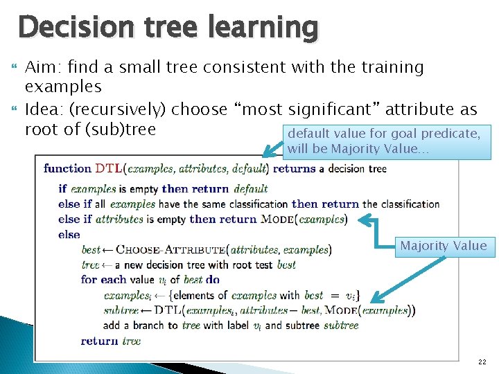
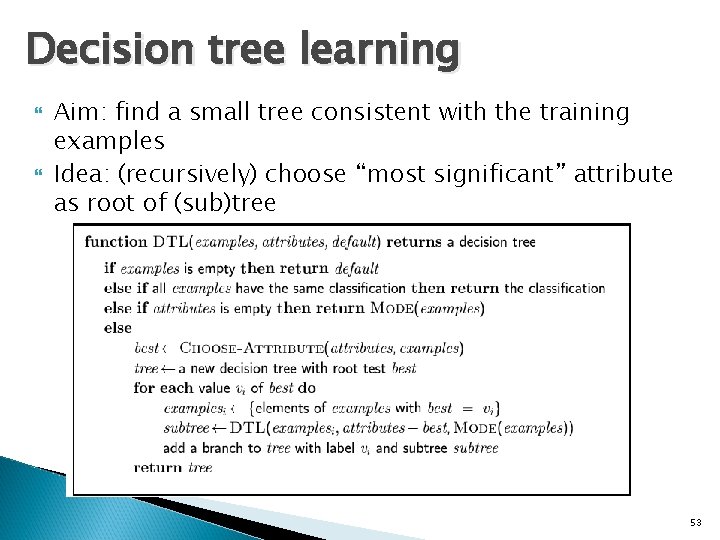
Decision tree learning Aim: find a small tree consistent with the training examples Idea: (recursively) choose “most significant” attribute as root of (sub)tree default value for goal predicate, will be Majority Value… Majority Value 22

Our Example 23

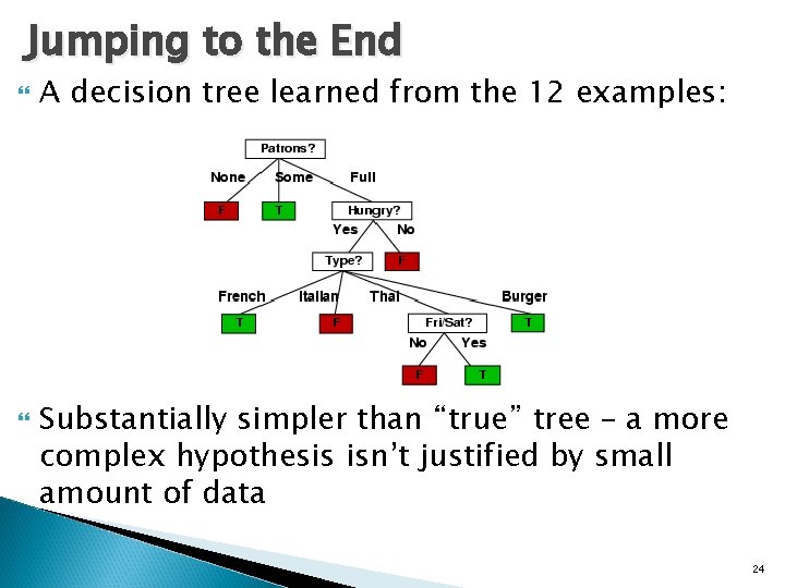
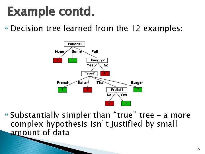
Jumping to the End A decision tree learned from the 12 examples: Substantially simpler than “true” tree – a more complex hypothesis isn’t justified by small amount of data 24

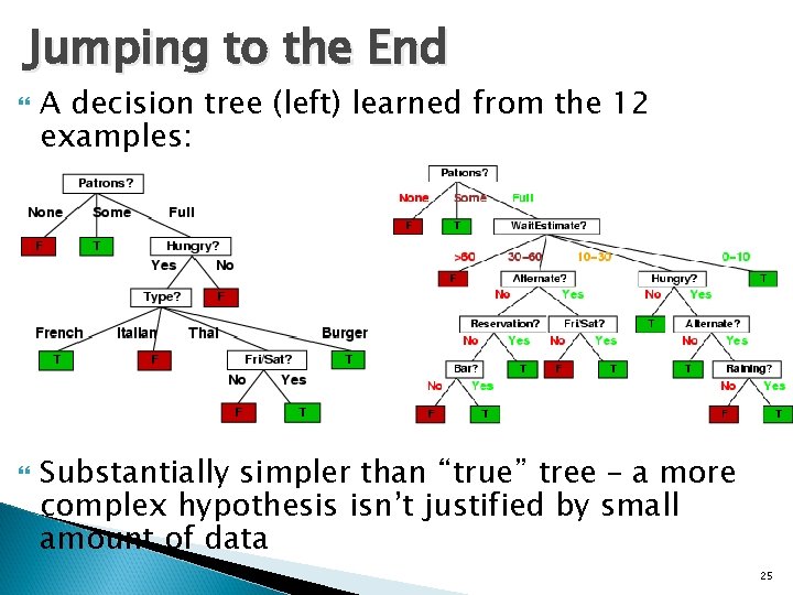
Jumping to the End A decision tree (left) learned from the 12 examples: Substantially simpler than “true” tree – a more complex hypothesis isn’t justified by small amount of data 25

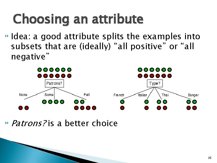
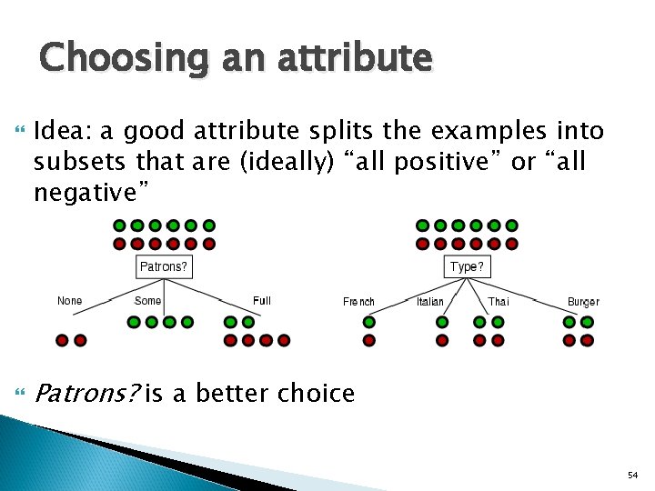
Choosing an attribute Idea: a good attribute splits the examples into subsets that are (ideally) “all positive” or “all negative” Patrons? is a better choice 26

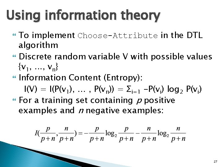
Using information theory To implement Choose-Attribute in the DTL algorithm Discrete random variable V with possible values {v 1, . . . , vn} Information Content (Entropy): I(V) = I(P(v 1), … , P(vn)) = Σi=1 -P(vi) log 2 P(vi) For a training set containing p positive examples and n negative examples: 27

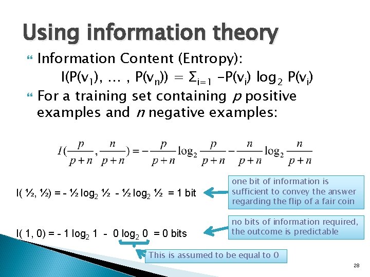
Using information theory Information Content (Entropy): I(P(v 1), … , P(vn)) = Σi=1 -P(vi) log 2 P(vi) For a training set containing p positive examples and n negative examples: I( ½, ½) = - ½ log 2 ½ = 1 bit I( 1, 0) = - 1 log 2 1 - 0 log 2 0 = 0 bits one bit of information is sufficient to convey the answer regarding the flip of a fair coin no bits of information required, the outcome is predictable This is assumed to be equal to 0 28

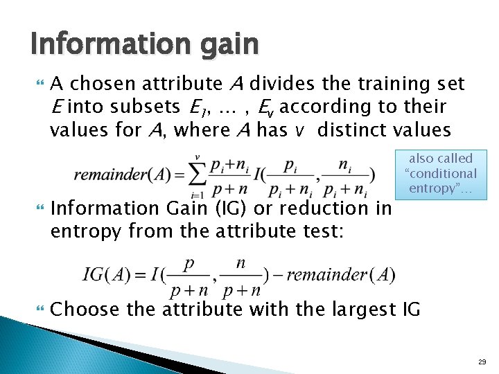
Information gain A chosen attribute A divides the training set E into subsets E 1, … , Ev according to their values for A, where A has v distinct values Information Gain (IG) or reduction in entropy from the attribute test: also called “conditional entropy”… Choose the attribute with the largest IG 29

Choosing an attribute Idea: a good attribute splits the examples into subsets that are (ideally) “all positive” or “all negative” Patrons? is a better choice 30

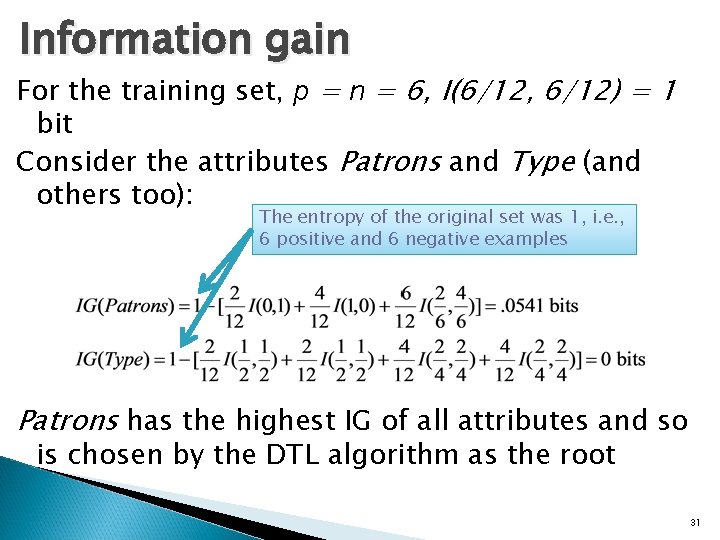
Information gain For the training set, p = n = 6, I(6/12, 6/12) = 1 bit Consider the attributes Patrons and Type (and others too): The entropy of the original set was 1, i. e. , 6 positive and 6 negative examples Patrons has the highest IG of all attributes and so is chosen by the DTL algorithm as the root 31

Note to other teachers and users of these slides. Andrew would be delighted if you found this source material useful in giving your own lectures. Feel free to use these slides verbatim, or to modify them to fit your own needs. Power. Point originals are available. If you make use of a significant portion of these slides in your own lecture, please include this message, or the following link to the source repository of Andrew’s tutorials: http: //www. cs. cmu. edu/~awm/tutorials. Comments and corrections gratefully received. Information Gain Andrew W. Moore Professor School of Computer Science Carnegie Mellon University www. cs. cmu. edu/~awm awm@cs. cmu. edu 412 -268 -7599

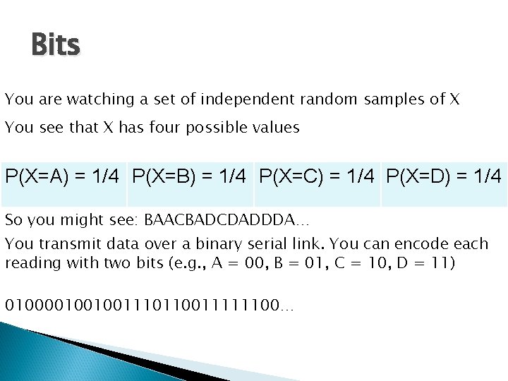
Bits You are watching a set of independent random samples of X You see that X has four possible values P(X=A) = 1/4 P(X=B) = 1/4 P(X=C) = 1/4 P(X=D) = 1/4 So you might see: BAACBADCDADDDA… You transmit data over a binary serial link. You can encode each reading with two bits (e. g. , A = 00, B = 01, C = 10, D = 11) 0100001001001110110011111100… 33

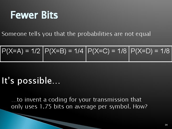
Fewer Bits Someone tells you that the probabilities are not equal P(X=A) = 1/2 P(X=B) = 1/4 P(X=C) = 1/8 P(X=D) = 1/8 It’s possible… …to invent a coding for your transmission that only uses 1. 75 bits on average per symbol. How? 34

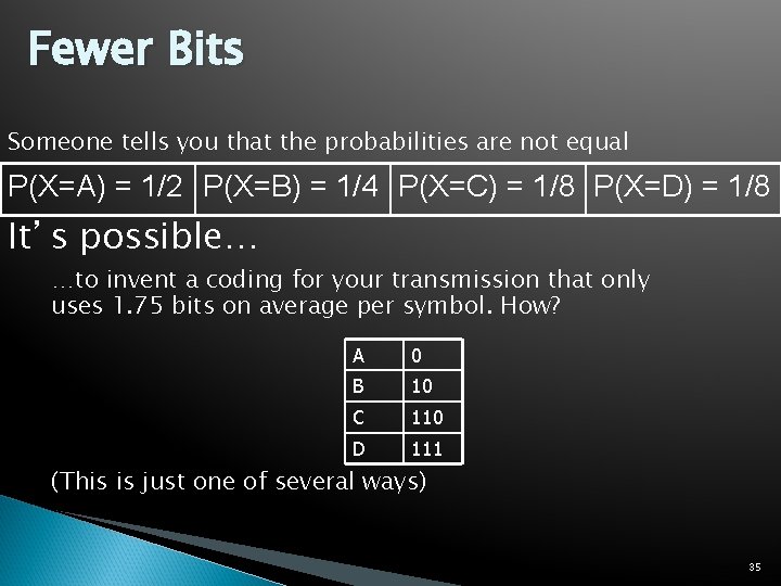
Fewer Bits Someone tells you that the probabilities are not equal P(X=A) = 1/2 P(X=B) = 1/4 P(X=C) = 1/8 P(X=D) = 1/8 It’s possible… …to invent a coding for your transmission that only uses 1. 75 bits on average per symbol. How? A 0 B 10 C 110 D 111 (This is just one of several ways) 35

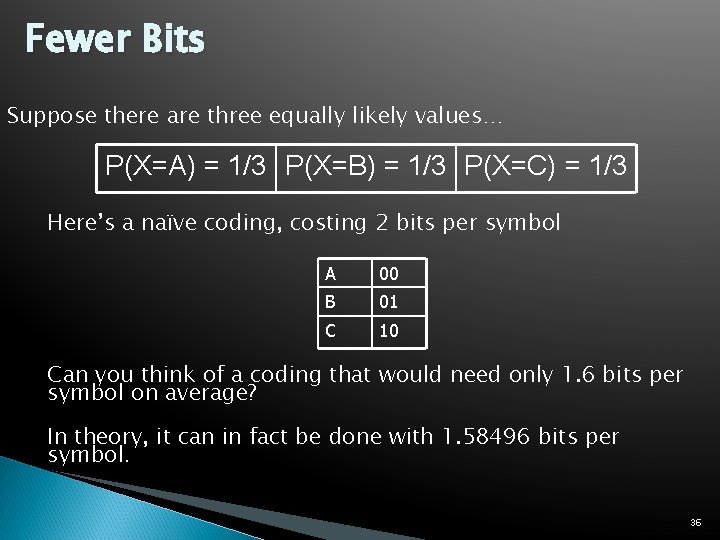
Fewer Bits Suppose there are three equally likely values… P(X=A) = 1/3 P(X=B) = 1/3 P(X=C) = 1/3 Here’s a naïve coding, costing 2 bits per symbol A 00 B 01 C 10 Can you think of a coding that would need only 1. 6 bits per symbol on average? In theory, it can in fact be done with 1. 58496 bits per symbol. 36

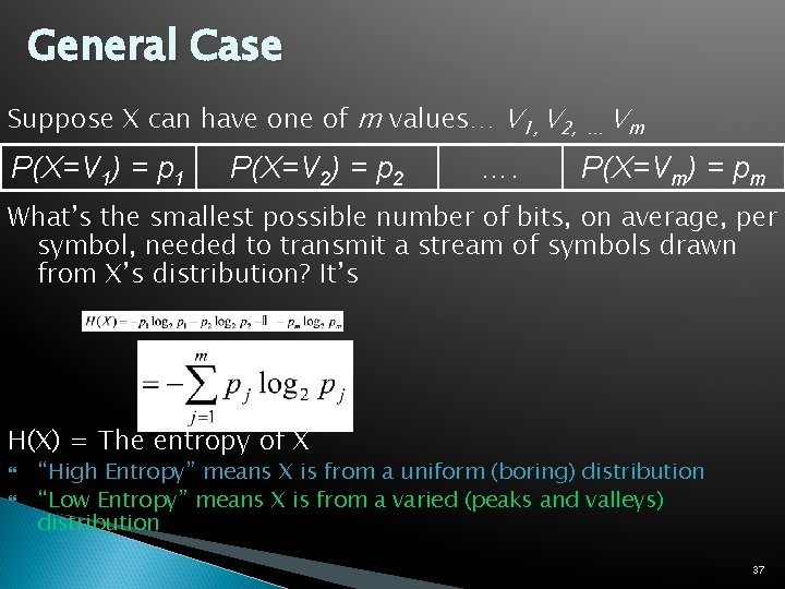
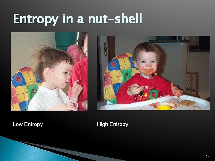
General Case Suppose X can have one of m values… V 1, V 2, … P(X=V 1) = p 1 P(X=Vm) = pm P(X=V 2) = p 2 …. Vm What’s the smallest possible number of bits, on average, per symbol, needed to transmit a stream of symbols drawn from X’s distribution? It’s H(X) = The entropy of X “High Entropy” means X is from a uniform (boring) distribution “Low Entropy” means X is from a varied (peaks and valleys) distribution 37

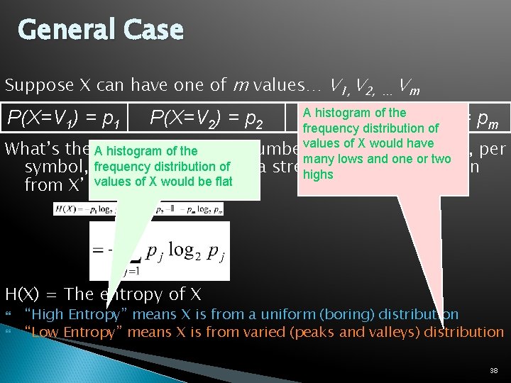
General Case Suppose X can have one of m values… V 1, V 2, … Vm A histogram of the …. P(X=V ) = pm frequency distribution ofm of X would have What’s the Asmallest numbervalues of bits, on average, per histogram ofpossible the many lows and one or two frequency distribution of symbol, needed to transmit a stream highsof symbols drawn of X would be. It’s flat from X’svalues distribution? P(X=V 1) = p 1 P(X=V 2) = p 2 H(X) = The entropy of X “High Entropy” means X is from a uniform (boring) distribution “Low Entropy” means X is from varied (peaks and valleys) distribution 38

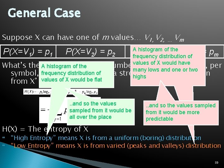
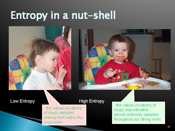
General Case Suppose X can have one of m values… V 1, V 2, … Vm A histogram of the …. P(X=V ) = pm frequency distribution ofm of X would have What’s the Asmallest numbervalues of bits, on average, per histogram ofpossible the many lows and one or two frequency distribution of symbol, needed to transmit a stream highsof symbols drawn of X would be. It’s flat from X’svalues distribution? P(X=V 1) = p 1 P(X=V 2) = p 2 . . and so the values sampled from it would be all over the place . . and so the values sampled from it would be more predictable H(X) = The entropy of X “High Entropy” means X is from a uniform (boring) distribution “Low Entropy” means X is from varied (peaks and valleys) distribution 39

Entropy in a nut-shell Low Entropy High Entropy 40

Entropy in a nut-shell Low Entropy High Entropy. . the values (locations of soup) sampled entirely from within the soup bowl . . the values (locations of soup) unpredictable. . . almost uniformly sampled throughout our dining room 41

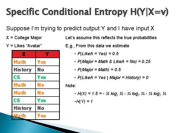
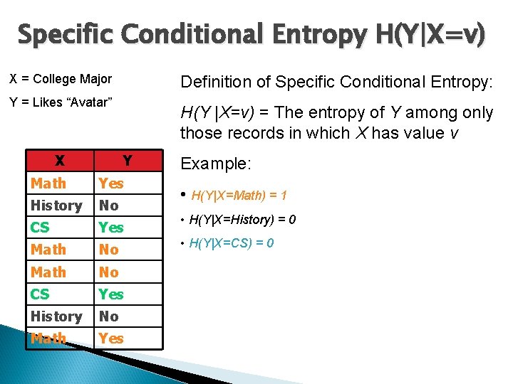
Specific Conditional Entropy H(Y|X=v) Suppose I’m trying to predict output Y and I have input X X = College Major Let’s assume this reflects the true probabilities Y = Likes “Avatar” E. g. , From this data we estimate X Y • P(Like. A = Yes) = 0. 5 Math Yes • P(Major = Math & Like. A = No) = 0. 25 History No • P(Major = Math) = 0. 5 CS Yes • P(Like. A = Yes | Major = History) = 0 Math No • H(X) = 1. 5 = - ½ log 2 ½ - ¼ log 2 ¼ CS Yes • H(Y) = 1 History No Math Yes Note:

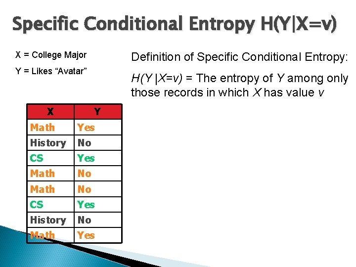
Specific Conditional Entropy H(Y|X=v) X = College Major Definition of Specific Conditional Entropy: Y = Likes “Avatar” X H(Y |X=v) = The entropy of Y among only those records in which X has value v Y Math Yes History No CS Yes Math No CS Yes History No Math Yes

Specific Conditional Entropy H(Y|X=v) X = College Major Definition of Specific Conditional Entropy: Y = Likes “Avatar” X H(Y |X=v) = The entropy of Y among only those records in which X has value v Y Math Yes History No CS Yes Math No CS Yes History No Math Yes Example: • H(Y|X=Math) = 1 • H(Y|X=History) = 0 • H(Y|X=CS) = 0

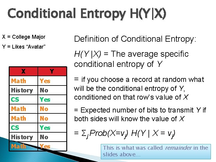
Conditional Entropy H(Y|X) X = College Major Definition of Conditional Entropy: Y = Likes “Avatar” X Y H(Y |X) = The average specific conditional entropy of Y Math Yes = if you choose a record at random what History No CS Yes will be the conditional entropy of Y, conditioned on that row’s value of X Math No CS Yes History No Math Yes = Expected number of bits to transmit Y if both sides will know the value of X = Σj Prob(X=vj) H(Y | X = vj) This is what was called remainder in the slides above…

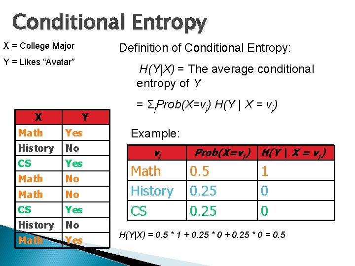
Conditional Entropy X = College Major Definition of Conditional Entropy: Y = Likes “Avatar” X H(Y|X) = The average conditional entropy of Y Y = Σj. Prob(X=vj) H(Y | X = vj) Math Yes Example: History No CS Yes vj Math No CS Yes History No Math Yes Math History CS Prob(X=vj) 0. 5 0. 25 H(Y | X = vj) 1 0 0 H(Y|X) = 0. 5 * 1 + 0. 25 * 0 = 0. 5

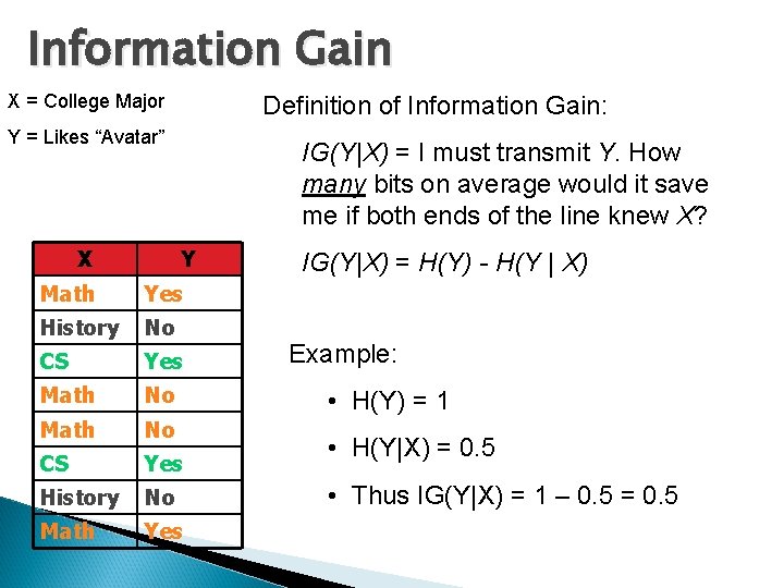
Information Gain X = College Major Definition of Information Gain: Y = Likes “Avatar” X IG(Y|X) = I must transmit Y. How many bits on average would it save me if both ends of the line knew X? Y Math Yes History No CS Yes Math No CS Yes History No Math Yes IG(Y|X) = H(Y) - H(Y | X) Example: • H(Y) = 1 • H(Y|X) = 0. 5 • Thus IG(Y|X) = 1 – 0. 5 = 0. 5

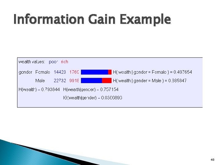
Information Gain Example 48

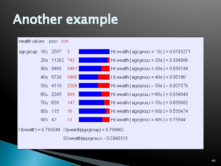
Another example 49

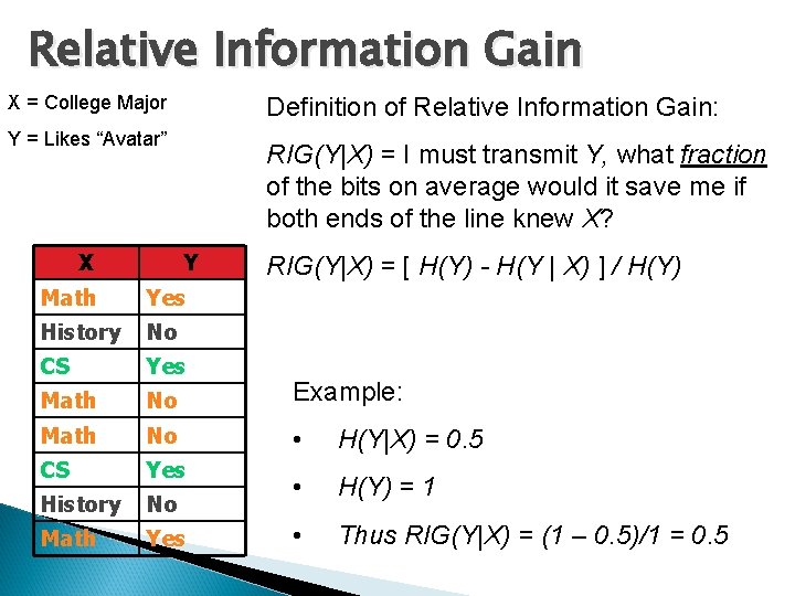
Relative Information Gain X = College Major Definition of Relative Information Gain: Y = Likes “Avatar” X RIG(Y|X) = I must transmit Y, what fraction of the bits on average would it save me if both ends of the line knew X? Y RIG(Y|X) = [ H(Y) - H(Y | X) ] / H(Y) Math Yes History No CS Yes Math No Example: Math No • H(Y|X) = 0. 5 CS Yes History No • H(Y) = 1 Math Yes • Thus RIG(Y|X) = (1 – 0. 5)/1 = 0. 5

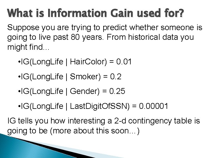
What is Information Gain used for? Suppose you are trying to predict whether someone is going to live past 80 years. From historical data you might find… • IG(Long. Life | Hair. Color) = 0. 01 • IG(Long. Life | Smoker) = 0. 2 • IG(Long. Life | Gender) = 0. 25 • IG(Long. Life | Last. Digit. Of. SSN) = 0. 00001 IG tells you how interesting a 2 -d contingency table is going to be (more about this soon…)

Decision trees One possible representation for hypotheses E. g. , here is the “true” tree for deciding whether to wait: 52

Decision tree learning Aim: find a small tree consistent with the training examples Idea: (recursively) choose “most significant” attribute as root of (sub)tree 53

Choosing an attribute Idea: a good attribute splits the examples into subsets that are (ideally) “all positive” or “all negative” Patrons? is a better choice 54

Example contd. Decision tree learned from the 12 examples: Substantially simpler than “true” tree – a more complex hypothesis isn’t justified by small amount of data 55

Performance measurement How do we know that h ≈ f ? Use theorems of computational/statistical learning theory (more on this, later) OR ◦ Randomly divide set of examples into training set and test set ◦ Learn h from training set ◦ Try h on test set of examples (measure percent of test set correctly classified) ◦ Repeat for: different sizes of training sets, and for each size of training set, different randomly selected sets 56

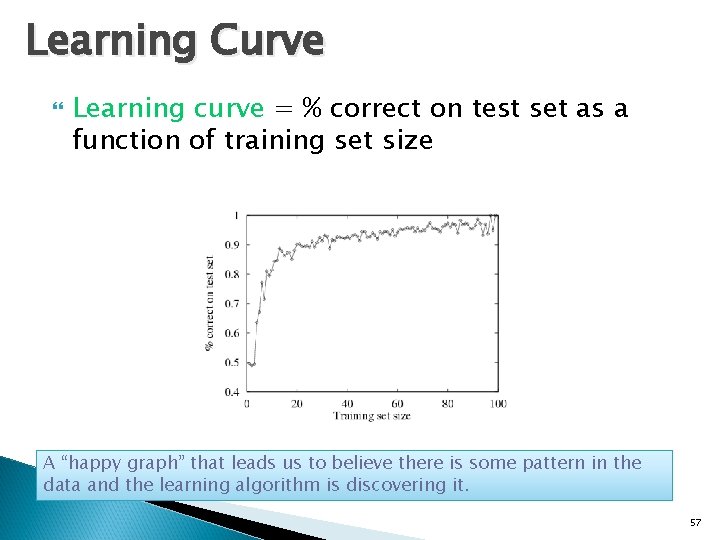
Learning Curve Learning curve = % correct on test set as a function of training set size A “happy graph” that leads us to believe there is some pattern in the data and the learning algorithm is discovering it. 57

No Peeking The learning algorithm cannot be allowed to “see” (or be influenced by) the test data before the hypothesis h is tested on it If we generate different h’s (for different parameters), and report back as our h the one that gave the best performance on the test set, then we’re allowing test set results to affect our learning algorithm This taints the results, but people do it anyway… 58

Summary Learning needed for unknown environments, lazy designers Learning agent = performance element + learning element For supervised learning, the aim is to find a simple hypothesis approximately consistent with training examples Decision tree learning using information gain Learning performance = prediction accuracy measured on test set 59

Note to other teachers and users of these slides. Andrew would be delighted if you found this source material useful in giving your own lectures. Feel free to use these slides verbatim, or to modify them to fit your own needs. Power. Point originals are available. If you make use of a significant portion of these slides in your own lecture, please include this message, or the following link to the source repository of Andrew’s tutorials: http: //www. cs. cmu. edu/~awm/tutorials. Comments and corrections gratefully received. Data Mining and Decision Trees Andrew W. Moore Professor School of Computer Science Carnegie Mellon University www. cs. cmu. edu/~awm awm@cs. cmu. edu 412 -268 -7599

Information Gain from Another Angle We’ll look at Information Gain, used both in Data Mining, and (again) in Decision Tree learning This gives us a new (reinforced) perspective on the topic 61

Outline Machine Learning Datasets What is Classification? Contingency Tables OLAP (Online Analytical Processing) What is Data Mining? Searching for High Information Gain Learning an unpruned decision tree recursively Training Set Error Test Set Error Overfitting Avoiding Overfitting 62

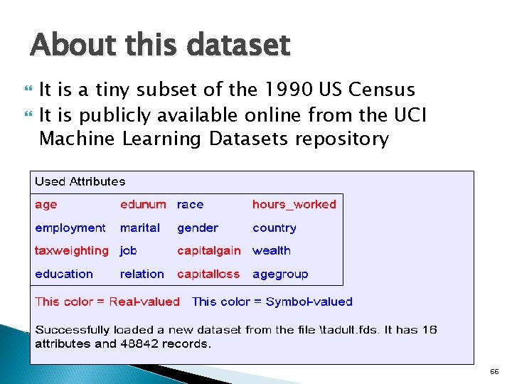
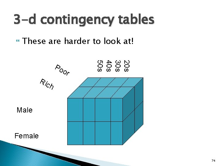
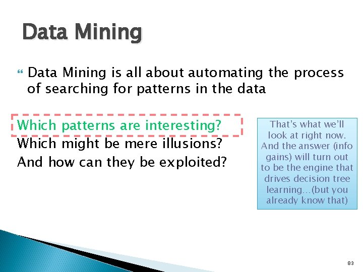
Here is a dataset 48, 842 records, 16 attributes [Kohavi 1995] 63

Outline Machine Learning Datasets What is Classification? Contingency Tables OLAP (Online Analytical Processing) What is Data Mining? Searching for High Information Gain Learning an unpruned decision tree recursively Training Set Error Test Set Error Overfitting Avoiding Overfitting 64

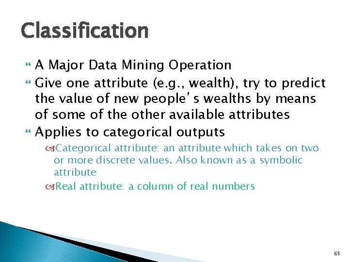
Classification A Major Data Mining Operation Give one attribute (e. g. , wealth), try to predict the value of new people’s wealths by means of some of the other available attributes Applies to categorical outputs Categorical attribute: an attribute which takes on two or more discrete values. Also known as a symbolic attribute Real attribute: a column of real numbers 65

About this dataset It is a tiny subset of the 1990 US Census It is publicly available online from the UCI Machine Learning Datasets repository 66

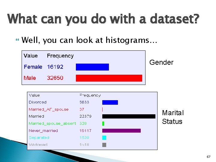
What can you do with a dataset? Well, you can look at histograms… Gender Marital Status 67

Outline Machine Learning Datasets What is Classification? Contingency Tables OLAP (Online Analytical Processing) What is Data Mining? Searching for High Information Gain Learning an unpruned decision tree recursively Training Set Error Test Set Error Overfitting Avoiding Overfitting 68

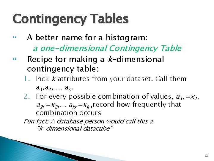
Contingency Tables A better name for a histogram: a one-dimensional Contingency Table Recipe for making a k-dimensional contingency table: 1. Pick k attributes from your dataset. Call them a 1, a 2, … ak. 2. For every possible combination of values, a 1, =x 1, a 2, =x 2, … ak, =xk , record how frequently that combination occurs Fun fact: A database person would call this a “k-dimensional datacube” 69

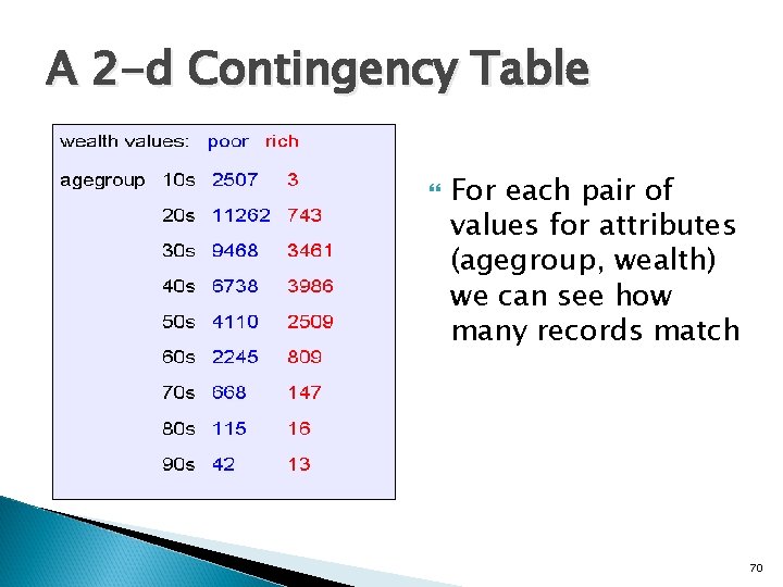
A 2 -d Contingency Table For each pair of values for attributes (agegroup, wealth) we can see how many records match 70

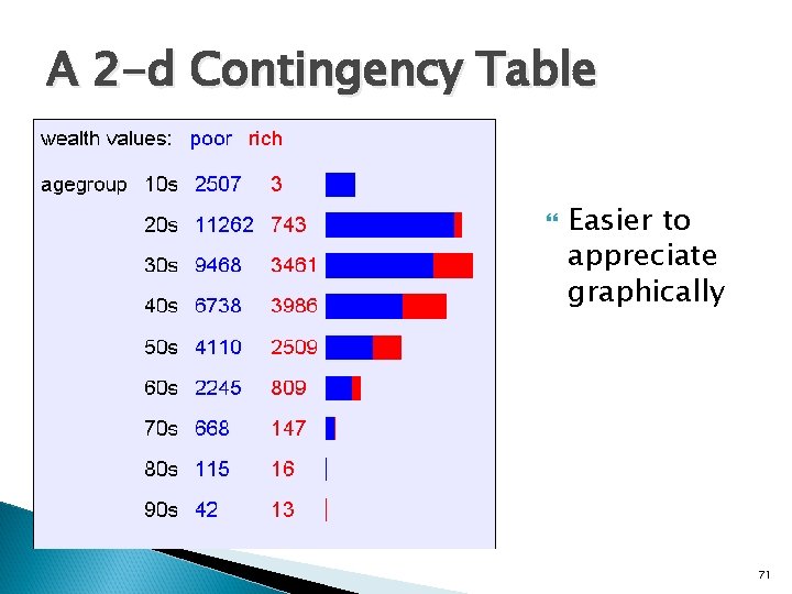
A 2 -d Contingency Table Easier to appreciate graphically 71

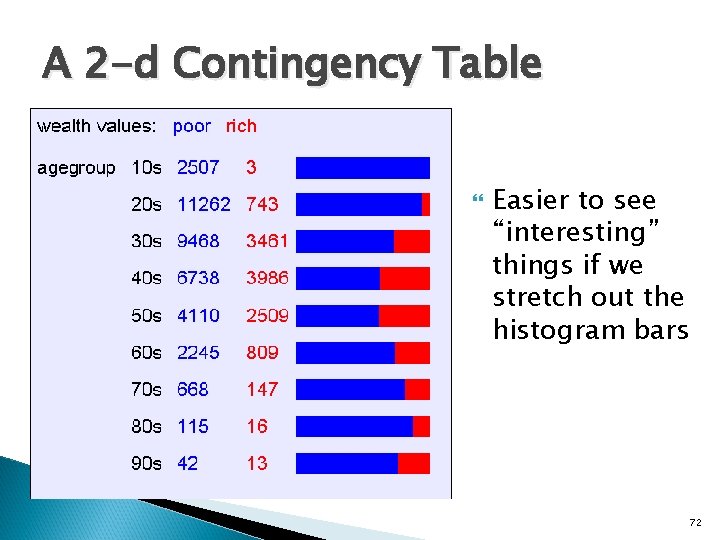
A 2 -d Contingency Table Easier to see “interesting” things if we stretch out the histogram bars 72

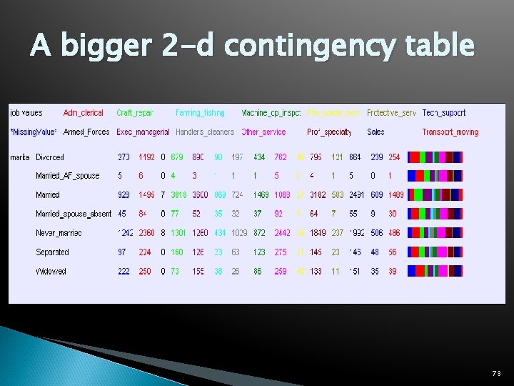
A bigger 2 -d contingency table 73

3 -d contingency tables These are harder to look at! Ric or 20 s 30 s 40 s 50 s Po h Male Female 74

Outline Machine Learning Datasets What is Classification? Contingency Tables OLAP (Online Analytical Processing) What is Data Mining? Searching for High Information Gain Learning an unpruned decision tree recursively Training Set Error Test Set Error Overfitting Avoiding Overfitting Information Gain of a real valued input Building Decision Trees with real Valued Inputs Andrew’s homebrewed hack: Binary Categorical Splits Example Decision Trees 75

On-Line Analytical Processing (OLAP) Software packages and database add-ons to do this are known as OLAP tools They usually include point and click navigation to view slices and aggregates of contingency tables They usually include nice histogram visualization 76

Time to stop and think Why would people want to look at contingency tables? 77

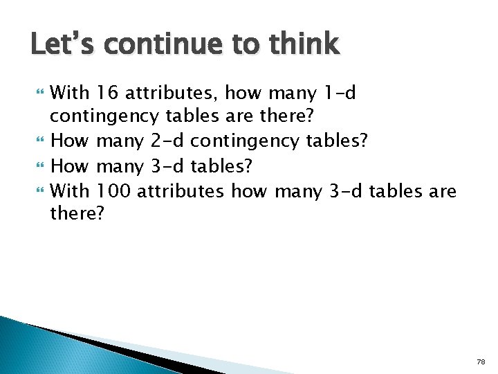
Let’s continue to think With 16 attributes, how many 1 -d contingency tables are there? How many 2 -d contingency tables? How many 3 -d tables? With 100 attributes how many 3 -d tables are there? 78

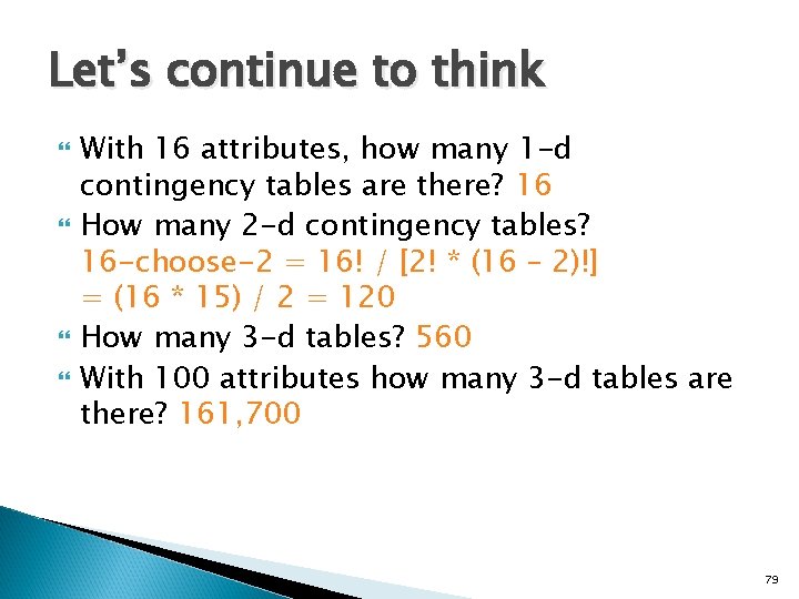
Let’s continue to think With 16 attributes, how many 1 -d contingency tables are there? 16 How many 2 -d contingency tables? 16 -choose-2 = 16! / [2! * (16 – 2)!] = (16 * 15) / 2 = 120 How many 3 -d tables? 560 With 100 attributes how many 3 -d tables are there? 161, 700 79

Manually looking at contingency tables Looking at one contingency table: can be as much fun as reading an interesting book Looking at ten tables: as much fun as watching CNN Looking at 100 tables: as much fun as watching an infomercial Looking at 100, 000 tables: as much fun as a three-week November vacation in Duluth with a dying weasel 80

Outline Machine Learning Datasets What is Classification? Contingency Tables OLAP (Online Analytical Processing) What is Data Mining? Searching for High Information Gain Learning an unpruned decision tree recursively Training Set Error Test Set Error Overfitting Avoiding Overfitting Information Gain of a real valued input Building Decision Trees with real Valued Inputs Andrew’s homebrewed hack: Binary Categorical Splits Example Decision Trees 81

Data Mining is all about automating the process of searching for patterns in the data Which patterns are interesting? Which might be mere illusions? And how can they be exploited? 82

Data Mining is all about automating the process of searching for patterns in the data Which patterns are interesting? Which might be mere illusions? And how can they be exploited? That’s what we’ll look at right now. And the answer (info gains) will turn out to be the engine that drives decision tree learning…(but you already know that) 83

Deciding whether a pattern is interesting We will use information theory A very large topic, originally used for compressing signals But more recently used for data mining… 84

Outline Machine Learning Datasets What is Classification? Contingency Tables OLAP (Online Analytical Processing) What is Data Mining? Searching for High Information Gain Learning an unpruned decision tree recursively Training Set Error Test Set Error Overfitting Avoiding Overfitting Information Gain of a real valued input Building Decision Trees with real Valued Inputs Andrew’s homebrewed hack: Binary Categorical Splits Example Decision Trees 85

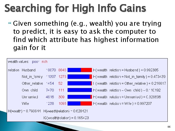
Searching for High Info Gains Given something (e. g. , wealth) you are trying to predict, it is easy to ask the computer to find which attribute has highest information gain for it 86

Outline Machine Learning Datasets What is Classification? Contingency Tables OLAP (Online Analytical Processing) What is Data Mining? Searching for High Information Gain Learning an unpruned decision tree recursively Training Set Error Test Set Error Overfitting Avoiding Overfitting 87

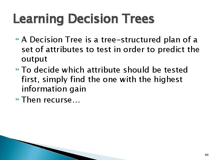
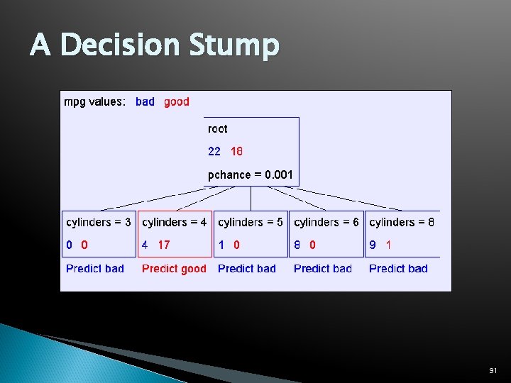
Learning Decision Trees A Decision Tree is a tree-structured plan of a set of attributes to test in order to predict the output To decide which attribute should be tested first, simply find the one with the highest information gain Then recurse… 88

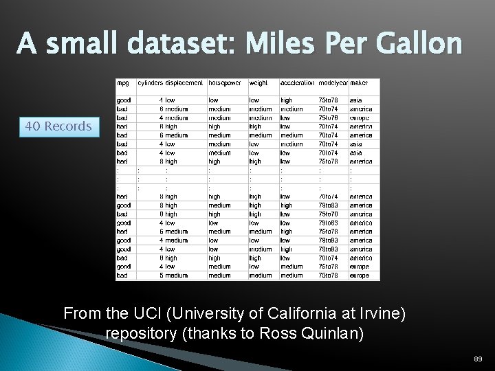
A small dataset: Miles Per Gallon 40 Records From the UCI (University of California at Irvine) repository (thanks to Ross Quinlan) 89

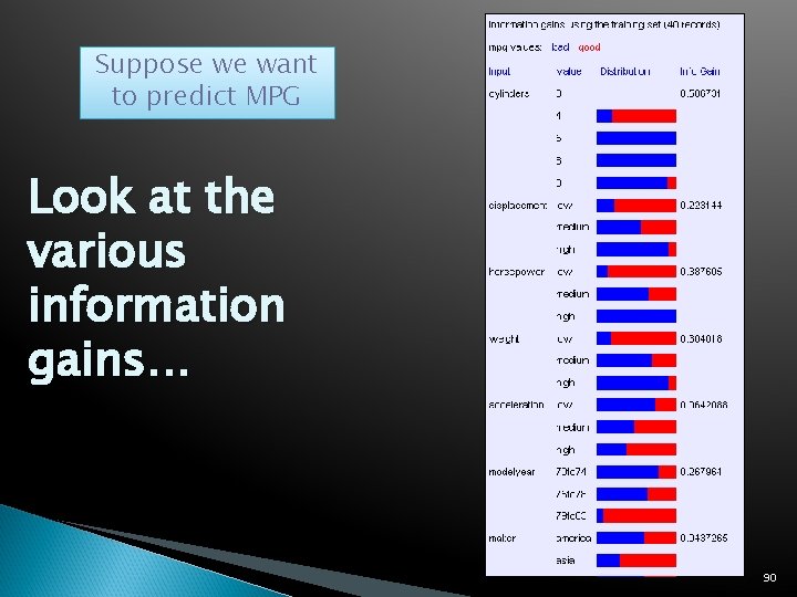
Suppose we want to predict MPG Look at the various information gains… 90

A Decision Stump 91

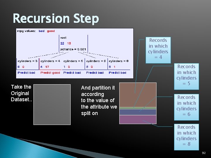
Recursion Step Records in which cylinders =4 Take the Original Dataset. . And partition it according to the value of the attribute we split on Records in which cylinders =5 Records in which cylinders =6 Records in which cylinders =8 92

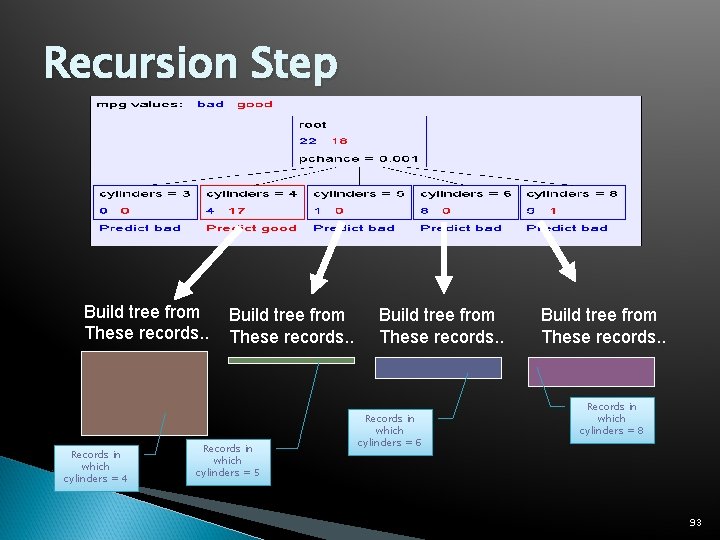
Recursion Step Build tree from These records. . Records in which cylinders = 4 Build tree from These records. . Records in which cylinders = 5 Build tree from These records. . Records in which cylinders = 6 Build tree from These records. . Records in which cylinders = 8 93

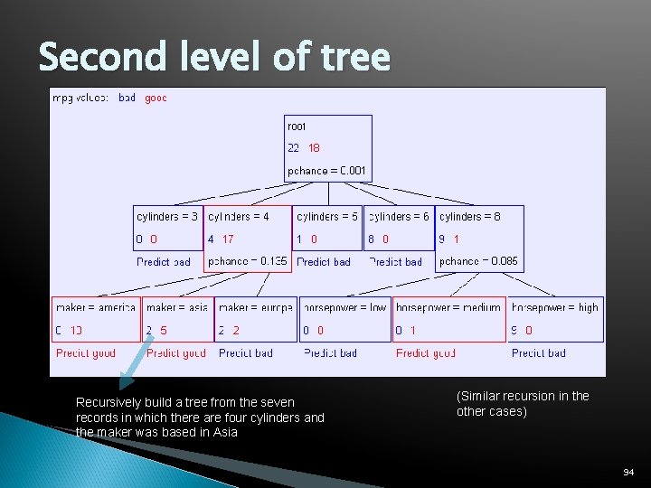
Second level of tree Recursively build a tree from the seven records in which there are four cylinders and the maker was based in Asia (Similar recursion in the other cases) 94

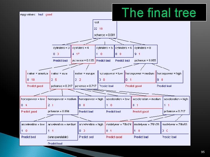
The final tree 95

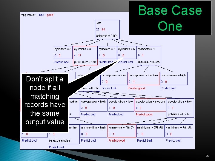
Base Case One Don’t split a node if all matching records have the same output value 96

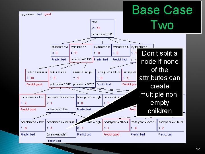
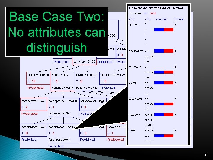
Base Case Two Don’t split a node if none of the attributes can create multiple nonempty children 97

Base Case Two: No attributes can distinguish 98

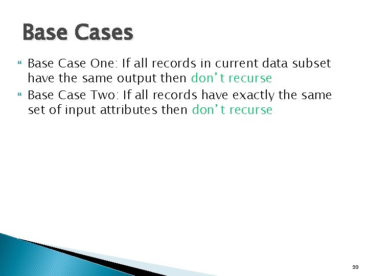
Base Cases Base Case One: If all records in current data subset have the same output then don’t recurse Base Case Two: If all records have exactly the same set of input attributes then don’t recurse 99

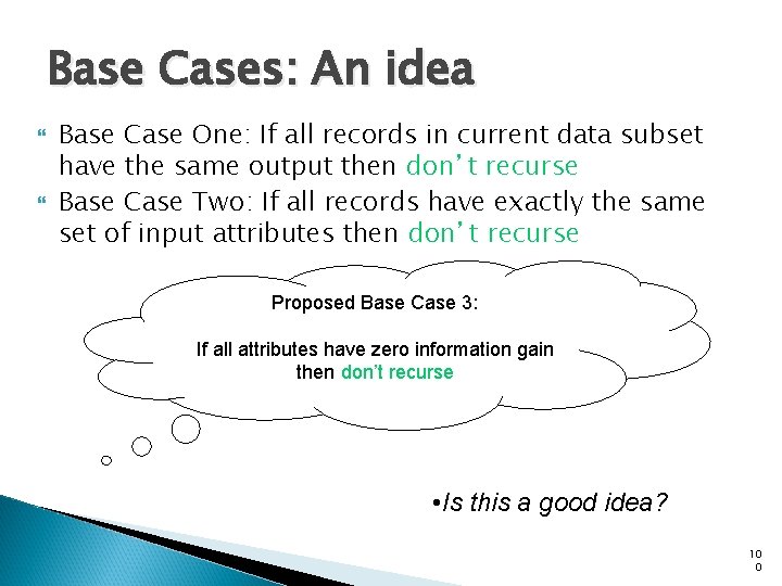
Base Cases: An idea Base Case One: If all records in current data subset have the same output then don’t recurse Base Case Two: If all records have exactly the same set of input attributes then don’t recurse Proposed Base Case 3: If all attributes have zero information gain then don’t recurse • Is this a good idea? 10 0

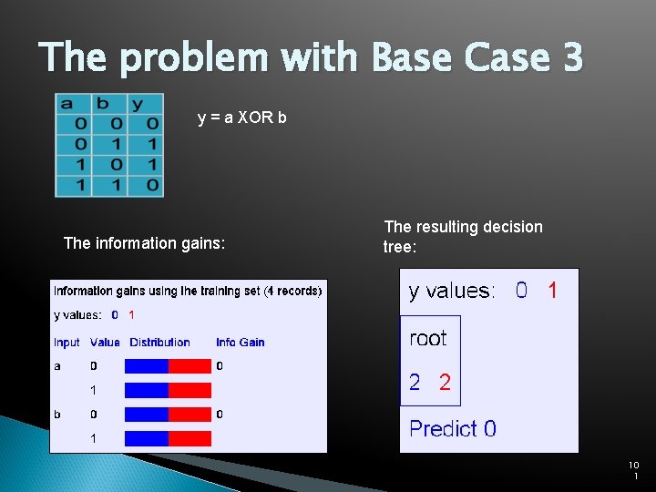
The problem with Base Case 3 y = a XOR b The information gains: The resulting decision tree: 10 1

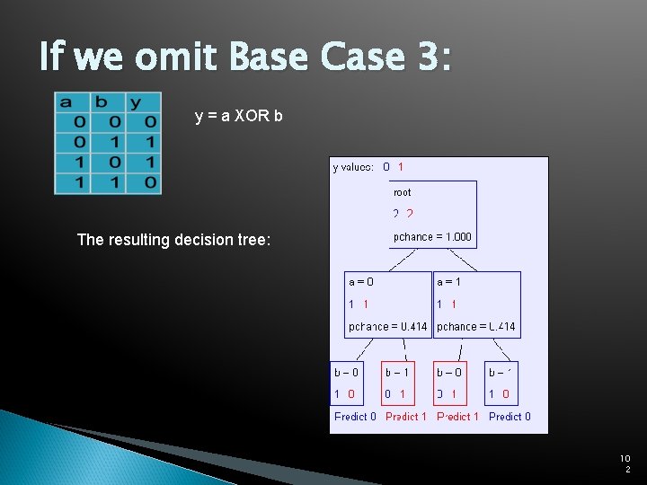
If we omit Base Case 3: y = a XOR b The resulting decision tree: 10 2

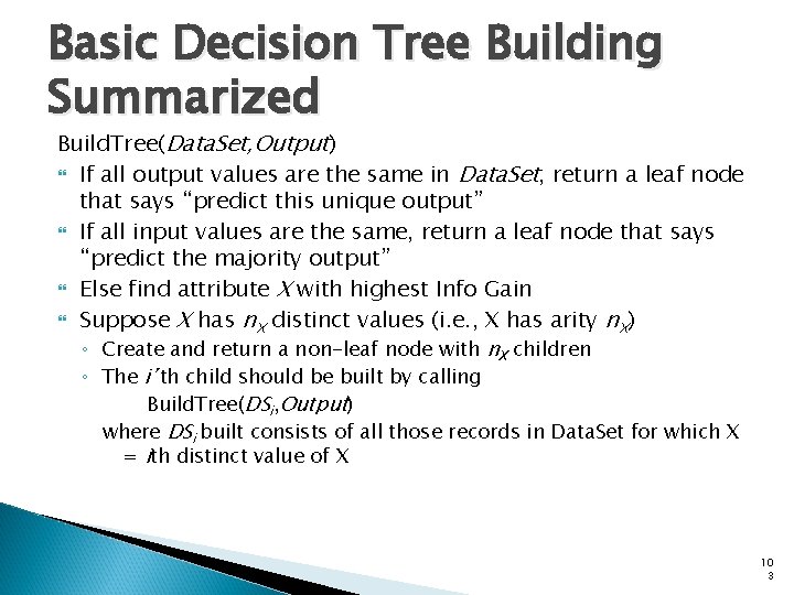
Basic Decision Tree Building Summarized Build. Tree(Data. Set, Output) If all output values are the same in Data. Set, return a leaf node that says “predict this unique output” If all input values are the same, return a leaf node that says “predict the majority output” Else find attribute X with highest Info Gain Suppose X has n. X distinct values (i. e. , X has arity n. X) ◦ Create and return a non-leaf node with n. X children ◦ The i’th child should be built by calling Build. Tree(DSi, Output) where DSi built consists of all those records in Data. Set for which X = ith distinct value of X 10 3

Outline Machine Learning Datasets What is Classification? Contingency Tables OLAP (Online Analytical Processing) What is Data Mining? Searching for High Information Gain Learning an unpruned decision tree recursively Training Set Error Test Set Error Overfitting Avoiding Overfitting 10 4

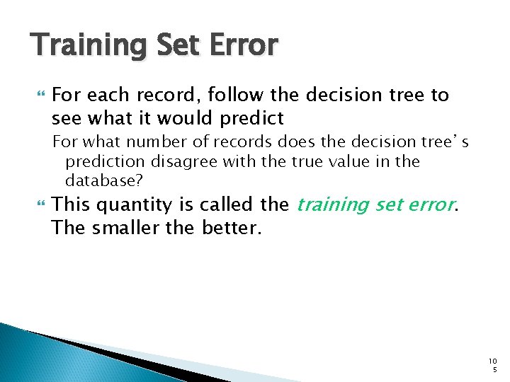
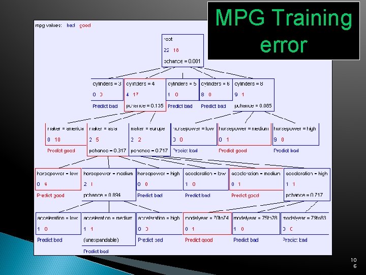
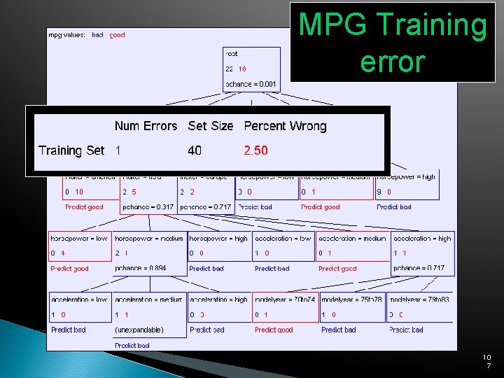
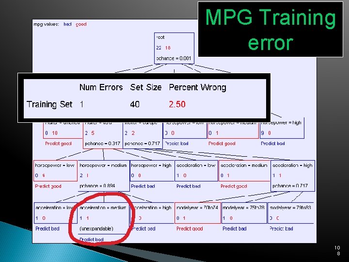
Training Set Error For each record, follow the decision tree to see what it would predict For what number of records does the decision tree’s prediction disagree with the true value in the database? This quantity is called the training set error. The smaller the better. 10 5

MPG Training error 10 6

MPG Training error 10 7

MPG Training error 10 8

Stop and reflect: Why are we doing this learning anyway? It is not usually in order to predict the training data’s output on data we have already seen 10 9

Stop and reflect: Why are we doing this learning anyway? It is not usually in order to predict the training data’s output on data we have already seen It is more commonly in order to predict the output value for future data we have not yet seen 11 0

Outline Machine Learning Datasets What is Classification? Contingency Tables OLAP (Online Analytical Processing) What is Data Mining? Searching for High Information Gain Learning an unpruned decision tree recursively Training Set Error Test Set Error Overfitting Avoiding Overfitting 11 1

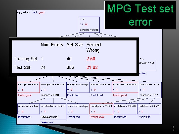
Test Set Error Suppose we are forward thinking We hide some data away when we learn the decision tree But once learned, we see how well the tree predicts that data This is a good simulation of what happens when we try to predict future data And it is called Test Set Error 11 2

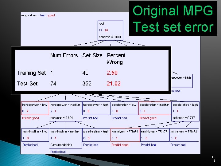
MPG Test set error 11 3

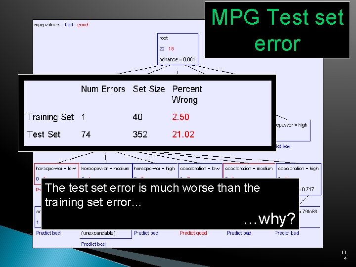
MPG Test set error The test set error is much worse than the training set error… …why? 11 4

Outline Machine Learning Datasets What is Classification? Contingency Tables OLAP (Online Analytical Processing) What is Data Mining? Searching for High Information Gain Learning an unpruned decision tree recursively Training Set Error Test Set Error Overfitting Avoiding Overfitting 11 5

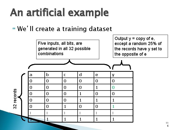
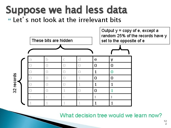
An artificial example We’ll create a training dataset Output y = copy of e, except a random 25% of the records have y set to the opposite of e 32 records Five inputs, all bits, are generated in all 32 possible combinations a b c d e y 0 0 0 0 0 1 1 1 0 0 1 : : : 1 1 1 11 6

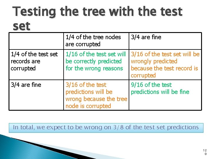
In our artificial example Suppose someone generates a test set according to the same method The test set is identical, except that some of the y’s will be different Some y’s that were corrupted in the training set will be uncorrupted in the testing set Some y’s that were uncorrupted in the training set will be corrupted in the test set 11 7

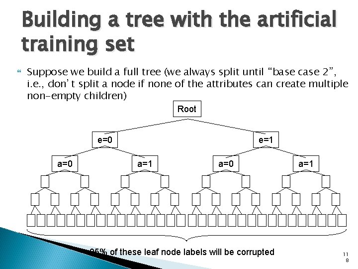
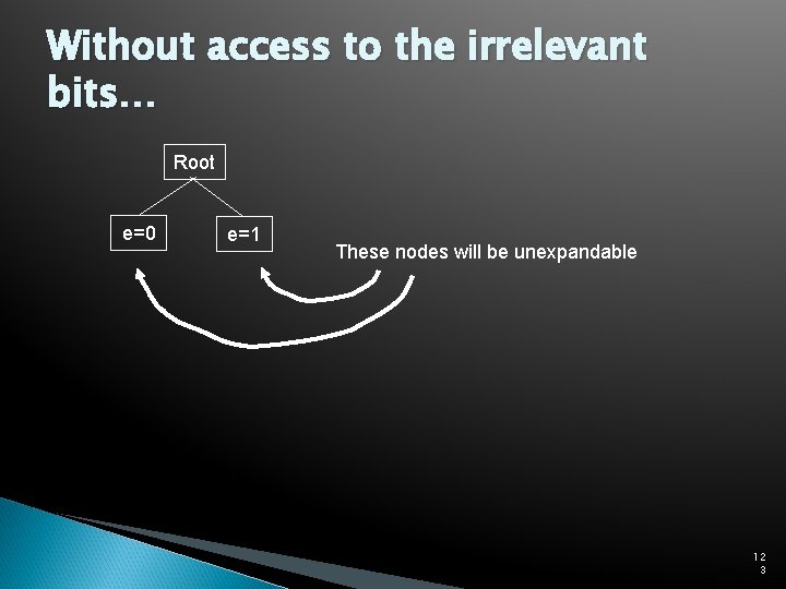
Building a tree with the artificial training set Suppose we build a full tree (we always split until “base case 2”, i. e. , don’t split a node if none of the attributes can create multiple non-empty children) Root e=0 a=0 e=1 a=0 25% of these leaf node labels will be corrupted a=1 11 8

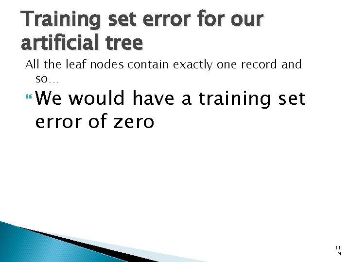
Training set error for our artificial tree All the leaf nodes contain exactly one record and so… We would have a training set error of zero 11 9

Testing the tree with the test set 1/4 of the tree nodes are corrupted 3/4 are fine 1/4 of the test set records are corrupted 1/16 of the test set will 3/16 of the test set will be be correctly predicted wrongly predicted for the wrong reasons because the test record is corrupted 3/4 are fine 3/16 of the test 9/16 of the test predictions will be fine wrong because the tree node is corrupted In total, we expect to be wrong on 3/8 of the test set predictions 12 0

What’s this example shown us? This explains the discrepancy between training and test set error But more importantly… …it indicates there’s something we should do about it if we want to predict well on future data 12 1

Suppose we had less data Let’s not look at the irrelevant bits Output y = copy of e, except a random 25% of the records have y set to the opposite of e These bits are hidden 32 records a b c d e y 0 0 0 0 0 1 1 1 0 0 1 : : : 1 1 1 What decision tree would we learn now? 12 2

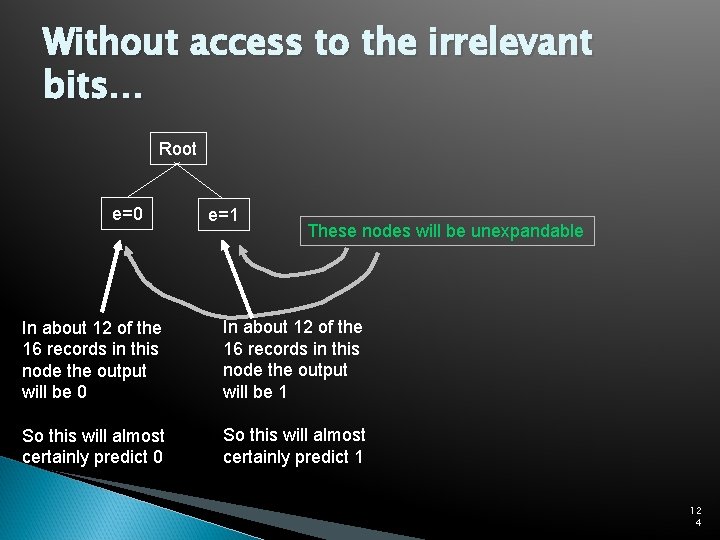
Without access to the irrelevant bits… Root e=0 e=1 These nodes will be unexpandable 12 3

Without access to the irrelevant bits… Root e=0 e=1 These nodes will be unexpandable In about 12 of the 16 records in this node the output will be 0 In about 12 of the 16 records in this node the output will be 1 So this will almost certainly predict 0 So this will almost certainly predict 1 12 4

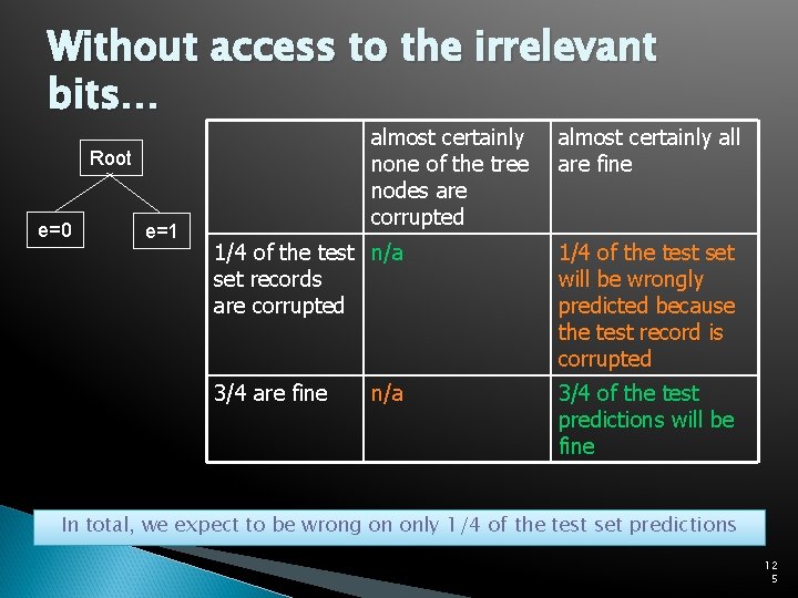
Without access to the irrelevant bits… almost certainly none of the tree nodes are corrupted Root e=0 e=1 almost certainly all are fine 1/4 of the test n/a set records are corrupted 1/4 of the test set will be wrongly predicted because the test record is corrupted 3/4 are fine 3/4 of the test predictions will be fine n/a In total, we expect to be wrong on only 1/4 of the test set predictions 12 5

Overfitting Definition: If your machine learning algorithm fits noise (i. e. , pays attention to parts of the data that are irrelevant) it is overfitting Fact (theoretical and empirical): If your machine learning algorithm is overfitting then it may perform less well on test set data 12 6

Outline Machine Learning Datasets What is Classification? Contingency Tables OLAP (Online Analytical Processing) What is Data Mining? Searching for High Information Gain Learning an unpruned decision tree recursively Training Set Error Test Set Error Overfitting Avoiding Overfitting 12 7

Avoiding overfitting Usually we do not know in advance which are the irrelevant variables …and it may depend on the context For example, if y = a AND b, then b is an irrelevant variable only in the portion of the tree in which a=0 But we can use simple statistics to warn us that we might be overfitting 12 8

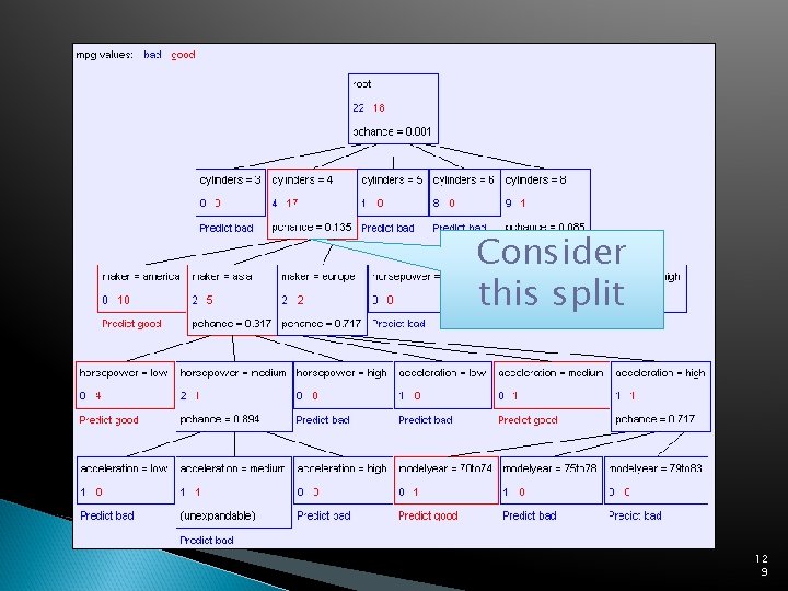
Consider this split 12 9

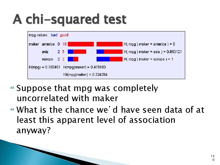
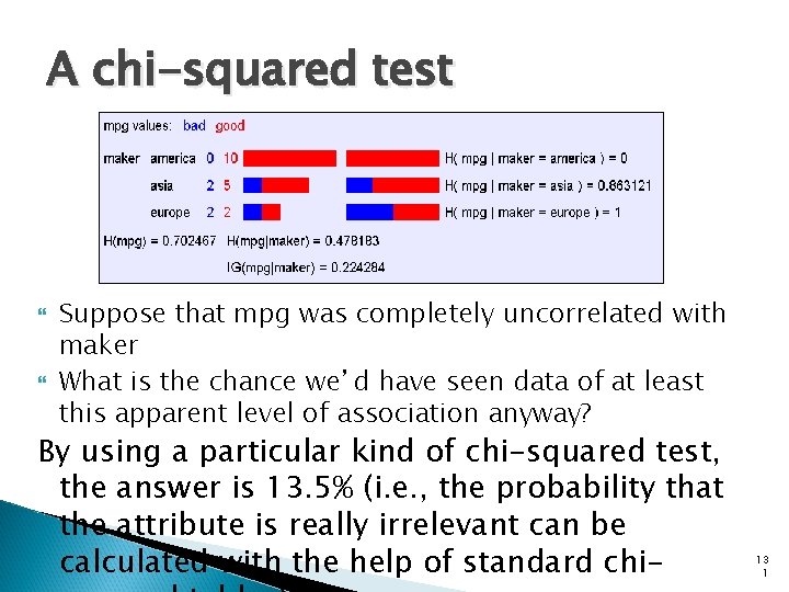
A chi-squared test Suppose that mpg was completely uncorrelated with maker What is the chance we’d have seen data of at least this apparent level of association anyway? 13 0

A chi-squared test Suppose that mpg was completely uncorrelated with maker What is the chance we’d have seen data of at least this apparent level of association anyway? By using a particular kind of chi-squared test, the answer is 13. 5% (i. e. , the probability that the attribute is really irrelevant can be calculated with the help of standard chi- 13 1

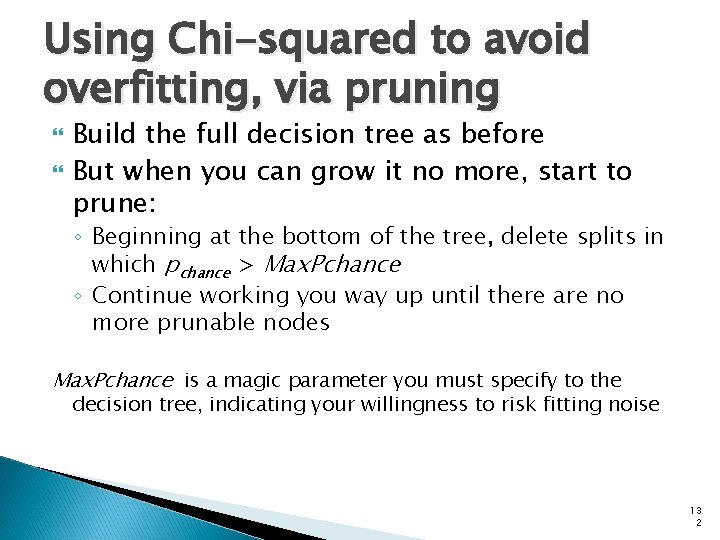
Using Chi-squared to avoid overfitting, via pruning Build the full decision tree as before But when you can grow it no more, start to prune: ◦ Beginning at the bottom of the tree, delete splits in which pchance > Max. Pchance ◦ Continue working you way up until there are no more prunable nodes Max. Pchance is a magic parameter you must specify to the decision tree, indicating your willingness to risk fitting noise 13 2

Original MPG Test set error 13 3

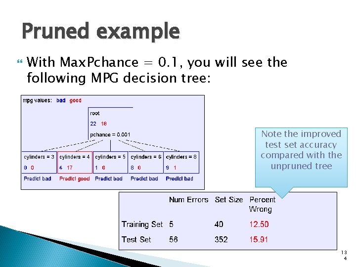
Pruned example With Max. Pchance = 0. 1, you will see the following MPG decision tree: Note the improved test set accuracy compared with the unpruned tree 13 4

Max. Pchance Good news: The decision tree can automatically adjust its pruning decisions according to the amount of apparent noise and data Bad news: The user must come up with a good value of Max. Pchance (note: Andrew Moore usually uses 0. 05, which is his favorite value for any magic parameter) Good news: But with extra work, the best Max. Pchance value can be estimated automatically by a technique called cross-validation 13 5

Cross-Validation Set aside some fraction of the known data and use it to test the prediction performance of a hypothesis induced from the remaining data K-fold cross-validation means that you run k experiments, each time setting aside a different 1/k of the data to test on, and average the results 13 6

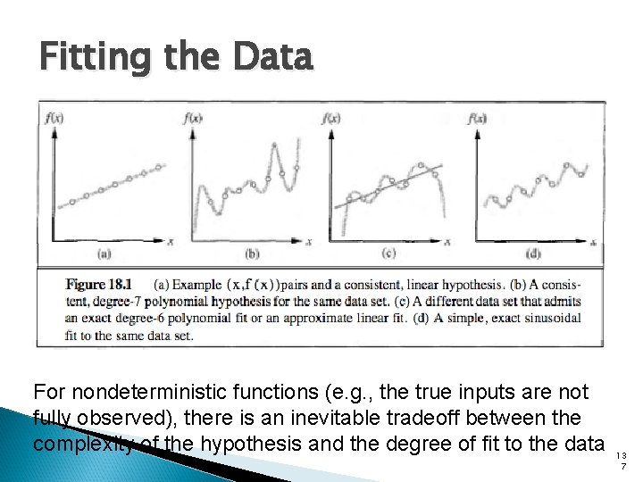
Fitting the Data For nondeterministic functions (e. g. , the true inputs are not fully observed), there is an inevitable tradeoff between the complexity of the hypothesis and the degree of fit to the data 13 7

Ensemble Learning Ensemble learning methods select a whole collection, or ensemble, of hypotheses from the hypothesis space and combine their predictions For example, we might generate a hundred different decision trees from the same training set, and have them vote on the best classification for a new example 13 8

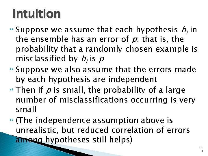
Intuition Suppose we assume that each hypothesis hi in the ensemble has an error of p; that is, the probability that a randomly chosen example is misclassified by hi is p Suppose we also assume that the errors made by each hypothesis are independent Then if p is small, the probability of a large number of misclassifications occurring is very small (The independence assumption above is unrealistic, but reduced correlation of errors among hypotheses still helps) 13 9

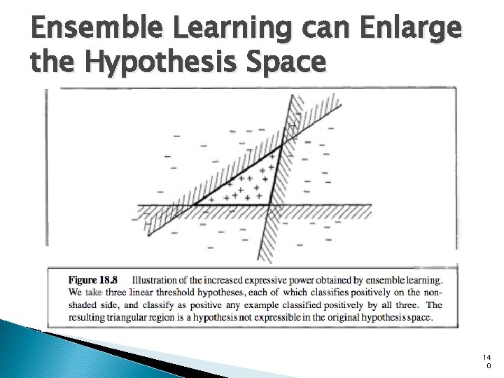
Ensemble Learning can Enlarge the Hypothesis Space 14 0

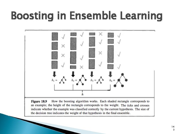
Boosting in Ensemble Learning In a weighted training set, each example has an associated weight w. J > 0; the higher the weight of an example, the higher the importance attached to it during the learning of a hypothesis Boosting starts with w. J = 1 for all the examples (i. e. , a normal training set) From this set, it generates the first hypothesis, h 1 This hypothesis will classify some of the training examples correctly and some incorrectly 14 1

Boosting in Ensemble Learning We want the next hypothesis to do better on the misclassified examples, so we increase their weights while decreasing the weights of the correctly classified examples From this new weighted training set, we generate hypothesis h 2 The process continues in this way until we have generated M hypotheses, where M is an input to the boosting algorithm The final ensemble hypothesis is a weightedmajority combination of all the M hypotheses, each weighted according to how well it performed on the training set 14 2

Boosting in Ensemble Learning 14 3

Boosting in Ensemble Learning There are many variants of the basic boosting idea with different ways of adjusting the weights and combining the hypotheses One specific algorithm, called Ada. Boost, is given in Russell and Norvig Ada. Boost has an important property: if the input learning algorithm L is a weak learning algorithm (that is, L always returns a hypothesis with weighted error on the training set that is slightly better than random guessing, i. e. , 50% for Boolean classification) then Ada. Boost will return a 14 4

Ada. Boost Thus, the algorithm boosts the accuracy of the original learning algorithm on the training data This result holds no matter how inexpressive the original hypothesis space and no matter how complex the function being learned 14 5

Learning Theory What can we say about the “correctness” of our learning procedure? Is there the possibility of exactly learning a concept? The answer is “yes”, but the technique is so restrictive, that it’s unusable in practice A stroll down memory lane… 14 6

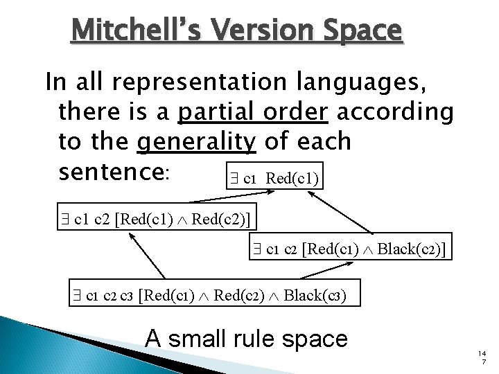
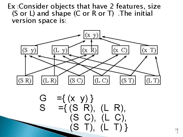
Mitchell’s Version Space In all representation languages, there is a partial order according to the generality of each sentence: $ c 1 Red(c 1) $ c 1 c 2 [Red(c 1) Red(c 2)] $ c 1 c 2 [Red(c 1) Black(c 2)] $ c 1 c 2 c 3 [Red(c 1) Red(c 2) Black(c 3) A small rule space 14 7

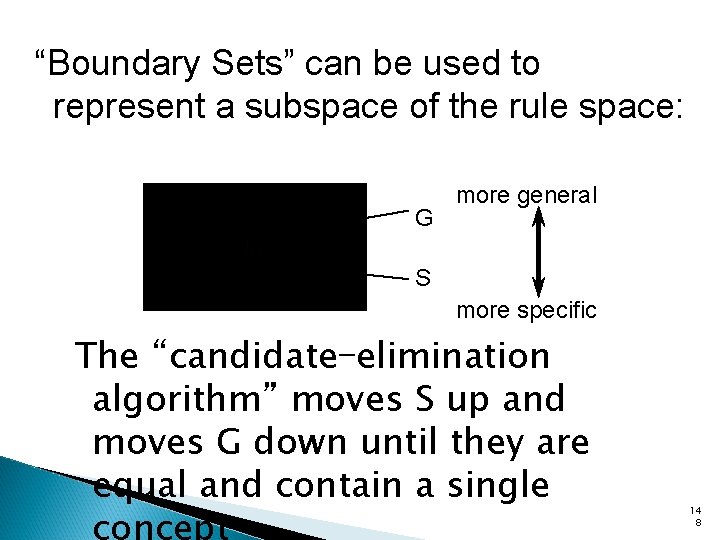
“Boundary Sets” can be used to represent a subspace of the rule space: G more general S more specific The “candidate-elimination algorithm” moves S up and moves G down until they are equal and contain a single 14 8

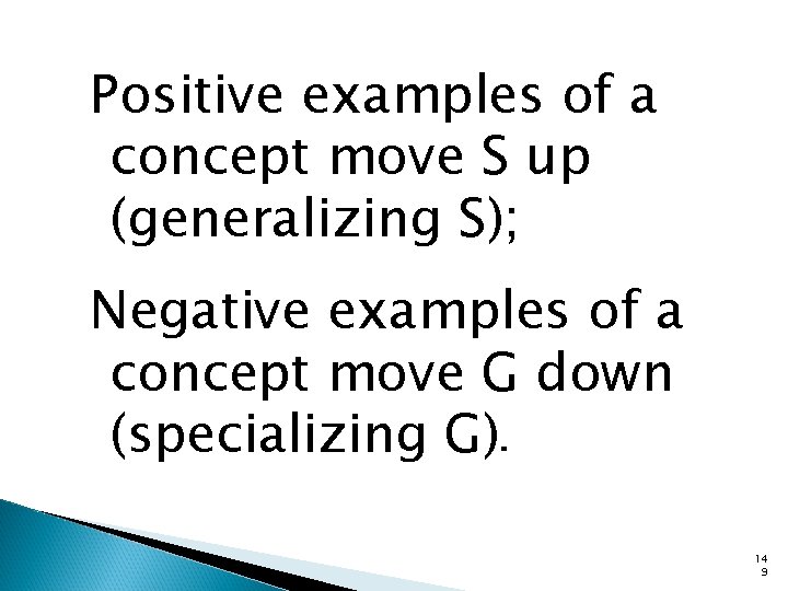
Positive examples of a concept move S up (generalizing S); Negative examples of a concept move G down (specializing G). 14 9

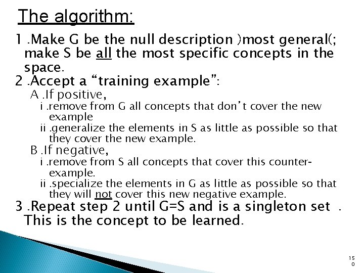
The algorithm: 1. Make G be the null description )most general(; make S be all the most specific concepts in the space. 2. Accept a “training example”: A. If positive, i. remove from G all concepts that don’t cover the new example ii. generalize the elements in S as little as possible so that they cover the new example. B. If negative, i. remove from S all concepts that cover this counterexample. ii. specialize the elements in G as little as possible so that they will not cover this new negative example. 3. Repeat step 2 until G=S and is a singleton set. This is the concept to be learned. 15 0

Ex : Consider objects that have 2 features, size (S or L) and shape (C or R or T). The initial version space is: (x y) (S R) (L y) (L R) G S (x R) (S C) (L C) (x C) (S T) ={ (x y) } ={ (S R), (L R), (S C), (L C), (S T), (L T) } (x T) (L T) 15 1

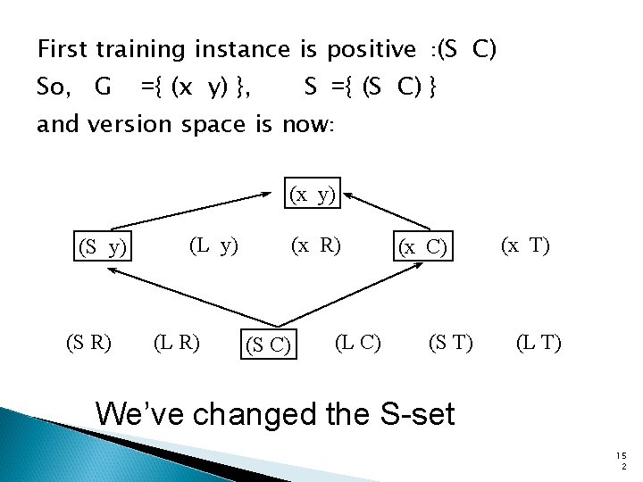
First training instance is positive : (S C) So, G ={ (x y) }, S ={ (S C) } and version space is now: (x y) (S R) (L y) (L R) (x R) (S C) (L C) (x C) (S T) (x T) (L T) We’ve changed the S-set 15 2

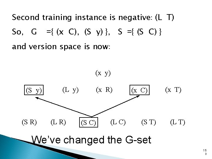
Second training instance is negative: (L T) So, G ={ (x C), (S y) }, S ={ (S C) } and version space is now: (x y) (S R) (L y) (L R) (x R) (S C) (L C) (x C) (S T) (x T) (L T) We’ve changed the G-set 15 3

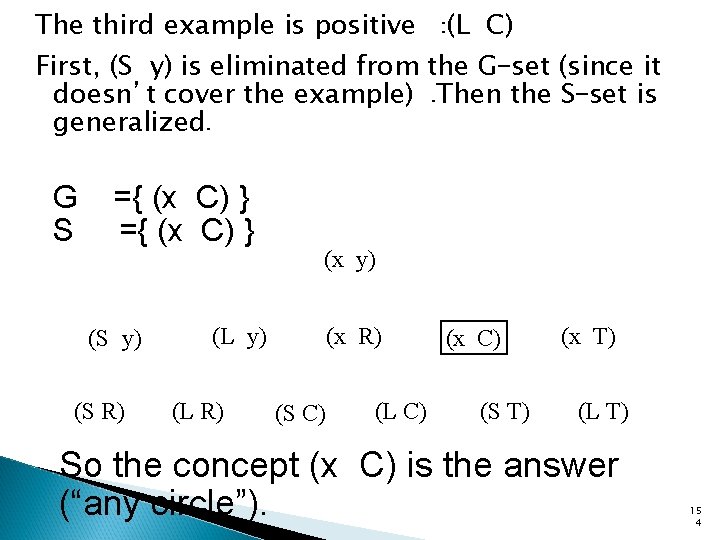
The third example is positive : (L C) First, (S y) is eliminated from the G-set (since it doesn’t cover the example). Then the S-set is generalized. G S ={ (x C) } (S y) (S R) (L y) (L R) (x y) (x R) (S C) (L C) (x C) (S T) (x T) (L T) So the concept (x C) is the answer (“any circle”). 15 4

Fatal Flaws Doesn’t tolerate news in the training set Doesn’t learn disjunctive concepts What is needed is a more general theory of learning that will approach the issue probabilistically, not deterministically Enter: PAC Learning 15 5

PAC Learning Intuition Any hypothesis that is seriously wrong will almost certainly be “found out” with high probability after a small number of examples, because it will make an incorrect prediction Thus, any hypothesis that is consistent with a sufficiently large set of training examples is unlikely to be seriously wrong: that is, it must be probably approximately correct 15 6

Stationarity Assumption The key assumption, called the stationarity assumption, is that the training and test sets are drawn randomly and independently from the same population of examples with the same probability distribution Without the stationarity assumption, theory can make no claims at all about the future, because there would be no necessary connection between future and past 15 7

How Many Examples Are Needed? Let X be the set of all possible examples Let D be the distribution from which examples are drawn Let H be the set of possible hypotheses Let N be the number of examples in the training set 15 8

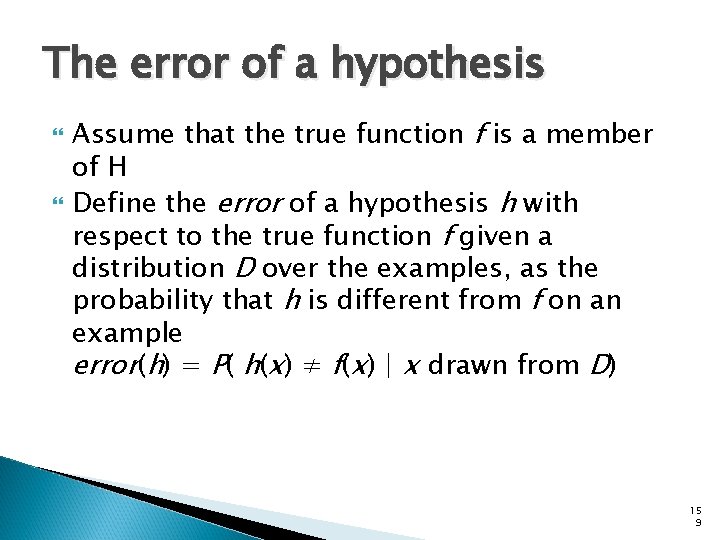
The error of a hypothesis Assume that the true function f is a member of H Define the error of a hypothesis h with respect to the true function f given a distribution D over the examples, as the probability that h is different from f on an example error(h) = P( h(x) ≠ f(x) | x drawn from D) 15 9

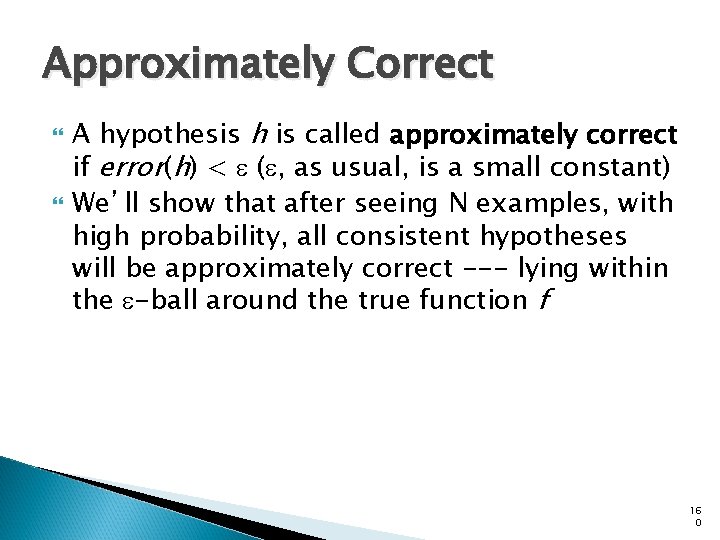
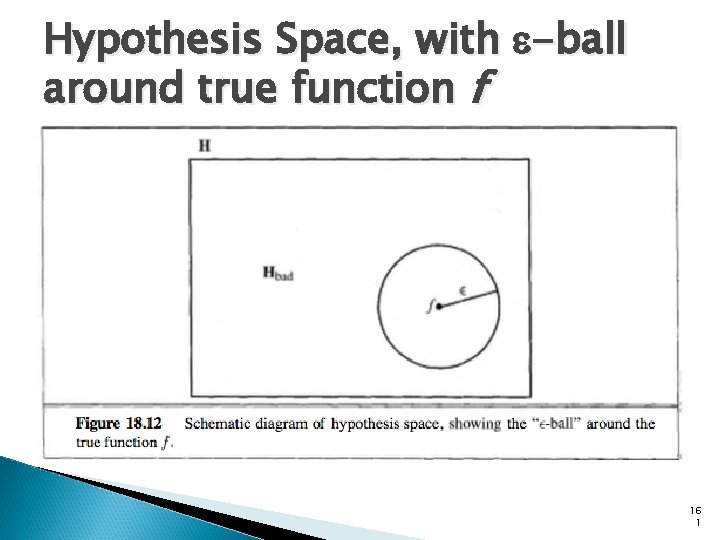
Approximately Correct A hypothesis h is called approximately correct if error(h) < e (e, as usual, is a small constant) We’ll show that after seeing N examples, with high probability, all consistent hypotheses will be approximately correct --- lying within the e-ball around the true function f 16 0

Hypothesis Space, with e-ball around true function f 16 1

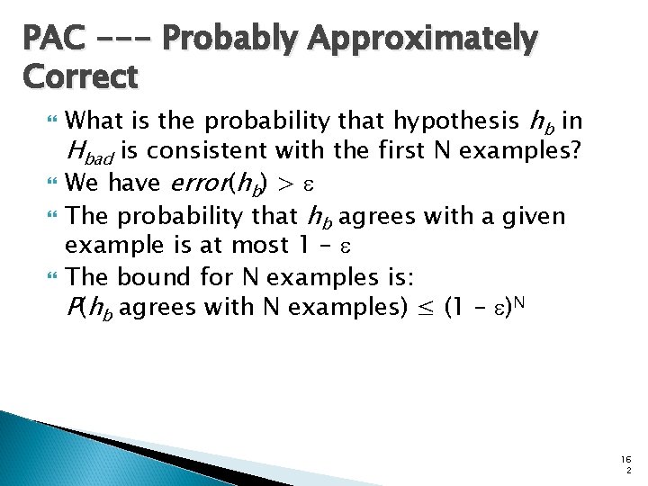
PAC --- Probably Approximately Correct What is the probability that hypothesis hb in Hbad is consistent with the first N examples? We have error(hb) > e The probability that hb agrees with a given example is at most 1 – e The bound for N examples is: P(hb agrees with N examples) ≤ (1 – e)N 16 2

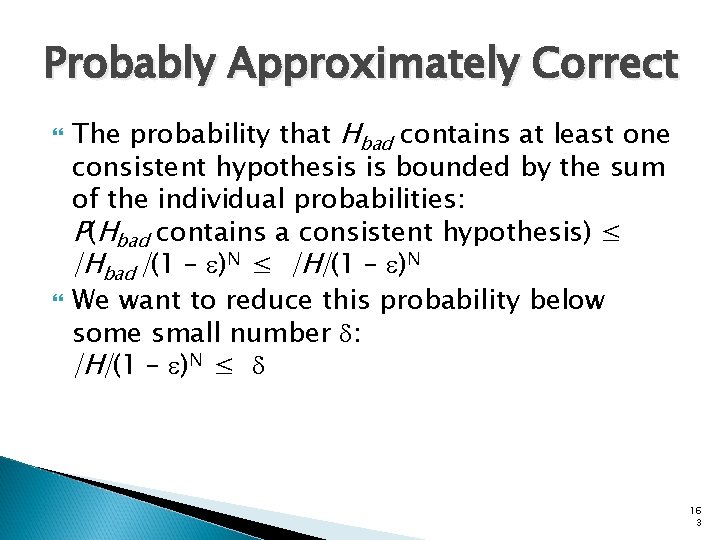
Probably Approximately Correct The probability that Hbad contains at least one consistent hypothesis is bounded by the sum of the individual probabilities: P(Hbad contains a consistent hypothesis) ≤ |Hbad |(1 – e)N ≤ |H|(1 – e)N We want to reduce this probability below some small number d: |H|(1 – e)N ≤ d 16 3

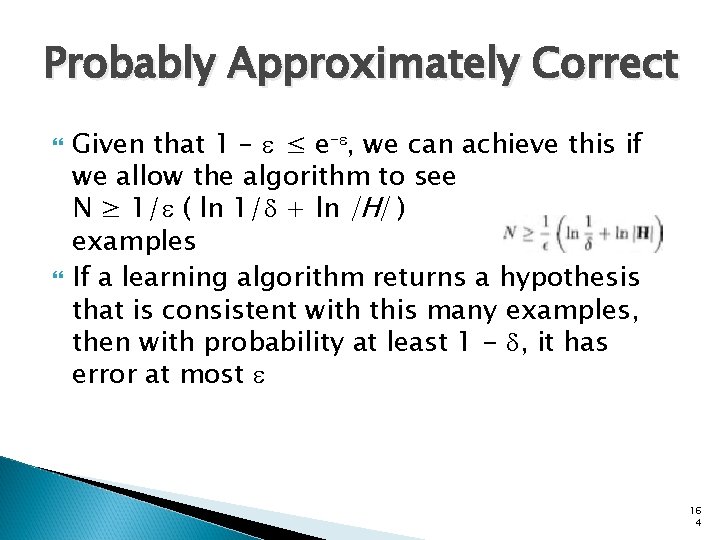
Probably Approximately Correct Given that 1 – e ≤ e–e, we can achieve this if we allow the algorithm to see N ≥ 1/e ( ln 1/d + ln |H| ) examples If a learning algorithm returns a hypothesis that is consistent with this many examples, then with probability at least 1 - d, it has error at most e 16 4

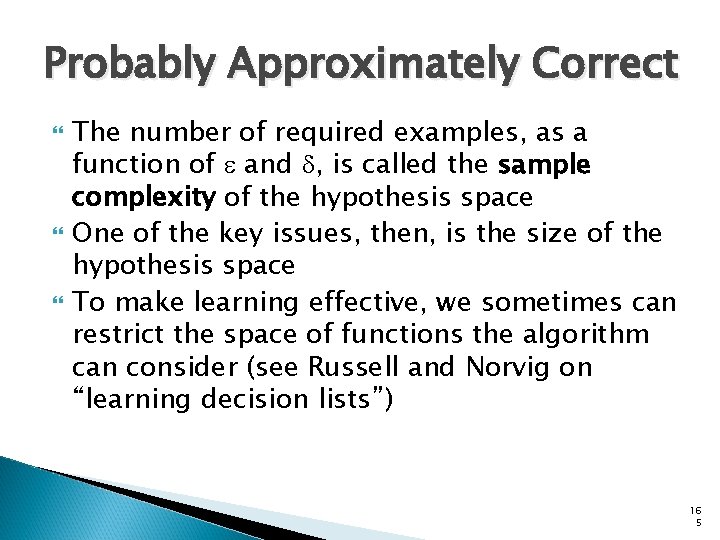
Probably Approximately Correct The number of required examples, as a function of e and d, is called the sample complexity of the hypothesis space One of the key issues, then, is the size of the hypothesis space To make learning effective, we sometimes can restrict the space of functions the algorithm can consider (see Russell and Norvig on “learning decision lists”) 16 5

Note to other teachers and users of these slides. Andrew would be delighted if you found this source material useful in giving your own lectures. Feel free to use these slides verbatim, or to modify them to fit your own needs. Power. Point originals are available. If you make use of a significant portion of these slides in your own lecture, please include this message, or the following link to the source repository of Andrew’s tutorials: http: //www. cs. cmu. edu/~awm/tutorials. Comments and corrections gratefully received. PAC-learning Andrew W. Moore Associate Professor School of Computer Science Carnegie Mellon University www. cs. cmu. edu/~awm awm@cs. cmu. edu 412 -268 -7599

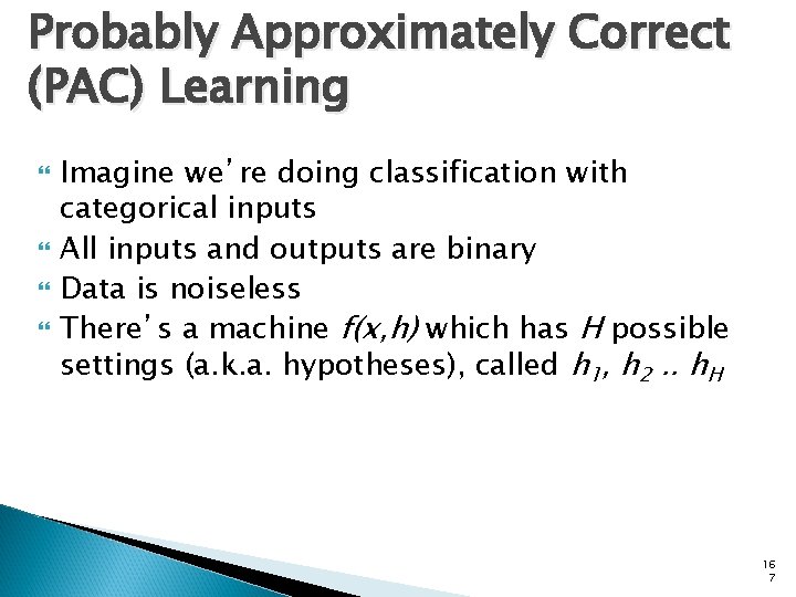
Probably Approximately Correct (PAC) Learning Imagine we’re doing classification with categorical inputs All inputs and outputs are binary Data is noiseless There’s a machine f(x, h) which has H possible settings (a. k. a. hypotheses), called h 1, h 2. . h. H 16 7

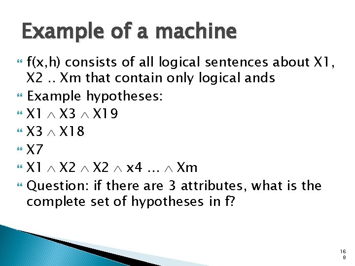
Example of a machine f(x, h) consists of all logical sentences about X 1, X 2. . Xm that contain only logical ands Example hypotheses: X 1 X 3 X 19 X 3 X 18 X 7 X 1 X 2 x 4 … Xm Question: if there are 3 attributes, what is the complete set of hypotheses in f? 16 8

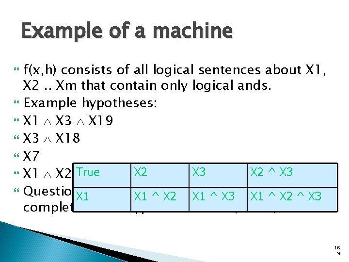
Example of a machine f(x, h) consists of all logical sentences about X 1, X 2. . Xm that contain only logical ands. Example hypotheses: X 1 X 3 X 19 X 3 X 18 X 7 X 2 ^ X 3 X 1 X 2 True X 2 x 4 X 2… Xm X 3 Question: are X 1 if there. X 1 ^3 X 2 attributes, X 1 ^ X 3 what X 1 ^ is X 2 the ^ X 3 complete set of hypotheses in f? (H = 8) 16 9

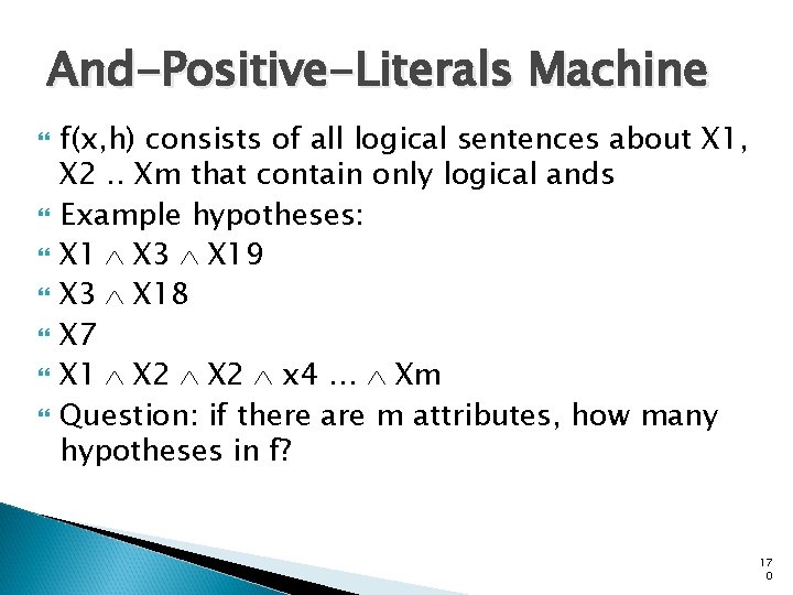
And-Positive-Literals Machine f(x, h) consists of all logical sentences about X 1, X 2. . Xm that contain only logical ands Example hypotheses: X 1 X 3 X 19 X 3 X 18 X 7 X 1 X 2 x 4 … Xm Question: if there are m attributes, how many hypotheses in f? 17 0

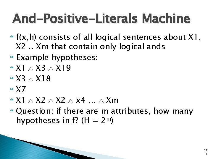
And-Positive-Literals Machine f(x, h) consists of all logical sentences about X 1, X 2. . Xm that contain only logical ands Example hypotheses: X 1 X 3 X 19 X 3 X 18 X 7 X 1 X 2 x 4 … Xm Question: if there are m attributes, how many hypotheses in f? (H = 2 m) 17 1

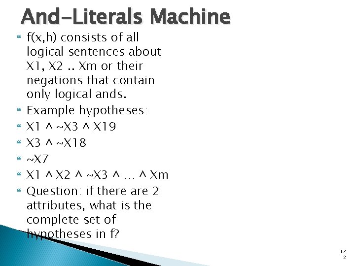
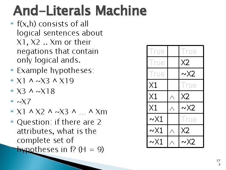
And-Literals Machine f(x, h) consists of all logical sentences about X 1, X 2. . Xm or their negations that contain only logical ands. Example hypotheses: X 1 ^ ~X 3 ^ X 19 X 3 ^ ~X 18 ~X 7 X 1 ^ X 2 ^ ~X 3 ^ … ^ Xm Question: if there are 2 attributes, what is the complete set of hypotheses in f? 17 2

And-Literals Machine f(x, h) consists of all logical sentences about X 1, X 2. . Xm or their negations that contain only logical ands. Example hypotheses: X 1 ^ ~X 3 ^ X 19 X 3 ^ ~X 18 ~X 7 X 1 ^ X 2 ^ ~X 3 ^ … ^ Xm Question: if there are 2 attributes, what is the complete set of hypotheses in f? (H = 9) True X 1 True X 2 ~X 2 True X 1 ~X 1 X 2 ~X 2 True X 2 ~X 2 17 3

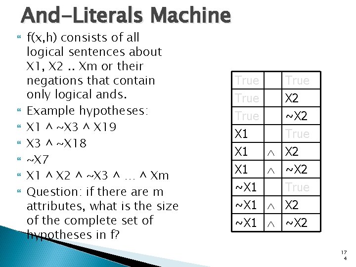
And-Literals Machine f(x, h) consists of all logical sentences about X 1, X 2. . Xm or their negations that contain only logical ands. Example hypotheses: X 1 ^ ~X 3 ^ X 19 X 3 ^ ~X 18 ~X 7 X 1 ^ X 2 ^ ~X 3 ^ … ^ Xm Question: if there are m attributes, what is the size of the complete set of hypotheses in f? True X 1 True X 2 ~X 2 True X 1 ~X 1 X 2 ~X 2 True X 2 ~X 2 17 4

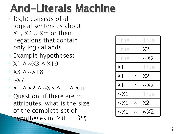
And-Literals Machine f(x, h) consists of all logical sentences about X 1, X 2. . Xm or their negations that contain only logical ands. Example hypotheses: X 1 ^ ~X 3 ^ X 19 X 3 ^ ~X 18 ~X 7 X 1 ^ X 2 ^ ~X 3 ^ … ^ Xm Question: if there are m attributes, what is the size of the complete set of hypotheses in f? (H = 3 m) True X 1 True X 2 ~X 2 True X 1 ~X 1 X 2 ~X 2 True X 2 ~X 2 17 5

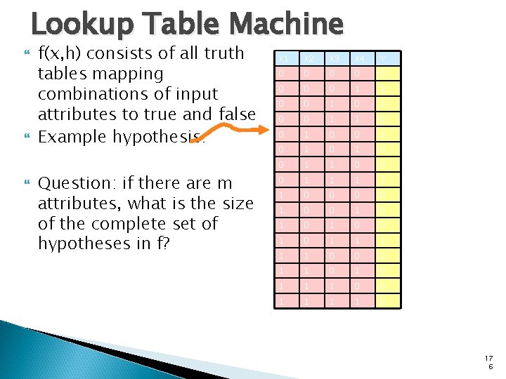
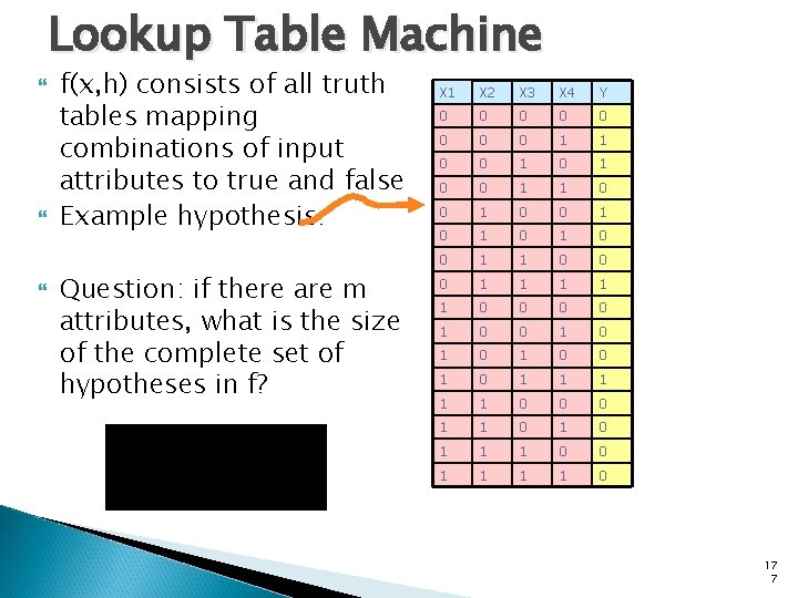
Lookup Table Machine f(x, h) consists of all truth tables mapping combinations of input attributes to true and false Example hypothesis: Question: if there are m attributes, what is the size of the complete set of hypotheses in f? X 1 X 2 X 3 X 4 Y 0 0 0 0 1 1 0 0 1 0 1 0 0 1 1 0 0 0 1 1 1 0 0 1 0 1 0 1 1 1 0 0 0 1 1 1 0 0 1 1 0 17 6

Lookup Table Machine f(x, h) consists of all truth tables mapping combinations of input attributes to true and false Example hypothesis: Question: if there are m attributes, what is the size of the complete set of hypotheses in f? X 1 X 2 X 3 X 4 Y 0 0 0 0 1 1 0 0 1 0 1 0 0 1 1 0 0 0 1 1 1 0 0 1 0 1 0 1 1 1 0 0 0 1 1 1 0 0 1 1 0 17 7

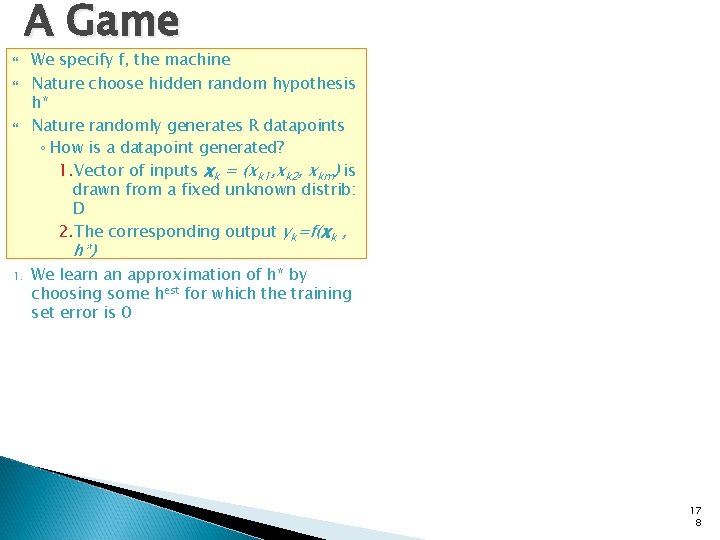
A Game We specify f, the machine Nature choose hidden random hypothesis h* Nature randomly generates R datapoints ◦ How is a datapoint generated? 1. Vector of inputs xk = (xk 1, xk 2, xkm) is drawn from a fixed unknown distrib: D 2. The corresponding output yk=f(xk , h*) 1. We learn an approximation of h* by choosing some hest for which the training set error is 0 17 8

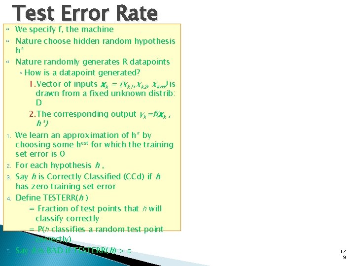
Test Error Rate We specify f, the machine Nature choose hidden random hypothesis h* Nature randomly generates R datapoints ◦ How is a datapoint generated? 1. Vector of inputs xk = (xk 1, xk 2, xkm) is drawn from a fixed unknown distrib: D 2. The corresponding output yk=f(xk , h*) 1. 2. 3. 4. 5. We learn an approximation of h* by choosing some hest for which the training set error is 0 For each hypothesis h , Say h is Correctly Classified (CCd) if h has zero training set error Define TESTERR(h ) = Fraction of test points that h will classify correctly = P(h classifies a random test point correctly) Say h is BAD if TESTERR(h) > e 17 9

Test Error Rate We specify f, the machine Nature choose hidden random hypothesis h* Nature randomly generates R datapoints ◦ How is a datapoint generated? 1. Vector of inputs xk = (xk 1, xk 2, xkm) is drawn from a fixed unknown distrib: D 2. The corresponding output yk=f(xk , h*) 1. 2. 3. 4. We learn an approximation of h* by choosing some hest for which the training set error is 0 For each hypothesis h , Say h is Correctly Classified (CCd) if h has zero training set error Define TESTERR(h ) = Fraction of test points that i will classify correctly = P(h classifies a random test point correctly) Say h is BAD if TESTERR(h) > e 18 0

Test Error Rate We specify f, the machine Nature choose hidden random hypothesis h* Nature randomly generates R datapoints ◦ How is a datapoint generated? 1. Vector of inputs xk = (xk 1, xk 2, xkm) is drawn from a fixed unknown distrib: D 2. The corresponding output yk=f(xk , h*) 1. 2. 3. 4. We learn an approximation of h* by choosing some hest for which the training set error is 0 For each hypothesis h , Say h is Correctly Classified (CCd) if h has zero training set error Define TESTERR(h ) = Fraction of test points that i will classify correctly = P(h classifies a random test point correctly) Say h is BAD if TESTERR(h) > e 18 1

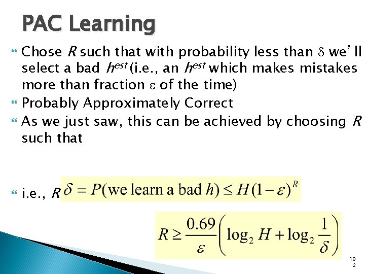
PAC Learning Chose R such that with probability less than d we’ll select a bad hest (i. e. , an hest which makes mistakes more than fraction e of the time) Probably Approximately Correct As we just saw, this can be achieved by choosing R such that i. e. , R such that 18 2

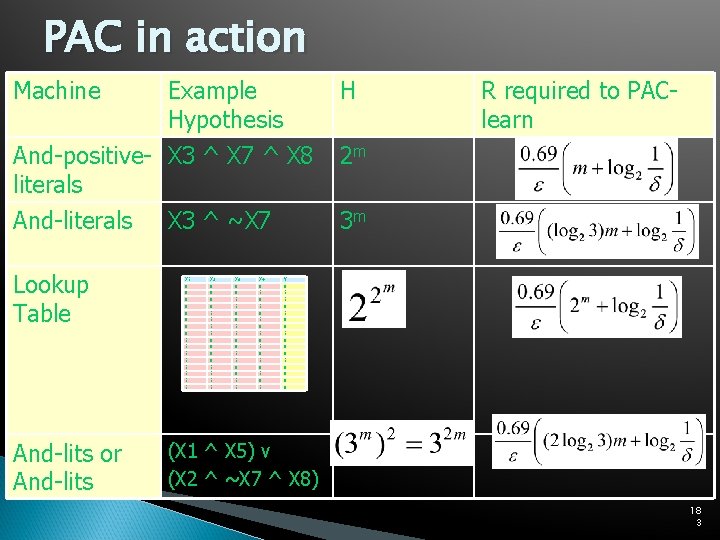
PAC in action Machine Example Hypothesis And-positive- X 3 ^ X 7 ^ X 8 literals H And-literals 3 m Lookup Table And-lits or And-lits X 3 ^ ~X 7 X 1 0 0 0 0 1 1 1 1 X 2 0 0 0 0 1 1 1 1 X 3 0 0 1 1 X 4 0 1 0 1 R required to PAClearn 2 m Y 0 1 1 0 0 0 0 (X 1 ^ X 5) v (X 2 ^ ~X 7 ^ X 8) 18 3

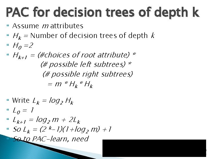
PAC for decision trees of depth k Assume m attributes Hk = Number of decision trees of depth k H 0 =2 Hk+1 = (#choices of root attribute) * (# possible left subtrees) * (# possible right subtrees) = m * H k * Hk Write Lk = log 2 Hk L 0 = 1 Lk+1 = log 2 m + 2 Lk So Lk = (2 k-1)(1+log 2 m) +1 So to PAC-learn, need 18 4