Hidden Markov Models Dave De Barr ddebarrgmu edu

Hidden Markov Models Dave De. Barr ddebarr@gmu. edu

Overview • General Characteristics • Simple Example • Speech Recognition

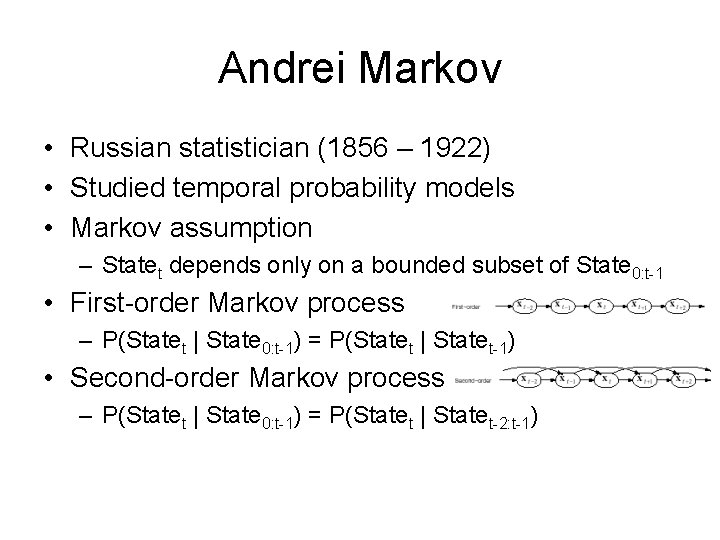
Andrei Markov • Russian statistician (1856 – 1922) • Studied temporal probability models • Markov assumption – Statet depends only on a bounded subset of State 0: t-1 • First-order Markov process – P(Statet | State 0: t-1) = P(Statet | Statet-1) • Second-order Markov process – P(Statet | State 0: t-1) = P(Statet | Statet-2: t-1)

Hidden Markov Model (HMM) • Evidence can be observed, but the state is hidden • Three components – Priors (initial state probabilities) – State transition model – Evidence observation model • Changes are assumed to be caused by a stationary process – The transition and observation models do not change

Simple HMM • Security guard resides in underground facility (with no way to see if it is raining) • Wants to determine the probability of rain given whether the director brings an umbrella • P(Rain 0 = t) = 0. 50

What can you do with an HMM? • Filtering – P(Statet | Evidence 1: t) • Prediction – P(Statet+k | Evidence 1: t) • Smoothing – P(Statek | Evidence 1: t) • Most likely explanation – argmax. State 1: t P(State 1: t | Evidence 1: t)

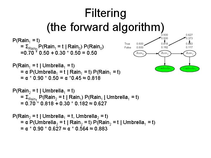
Filtering (the forward algorithm) P(Rain 1 = t) = ΣRain 0 P(Rain 1 = t | Rain 0) P(Rain 0) =0. 70 * 0. 50 + 0. 30 * 0. 50 = 0. 50 P(Rain 1 = t | Umbrella 1 = t) = α P(Umbrella 1 = t | Rain 1 = t) P(Rain 1 = t) = α * 0. 90 * 0. 50 = α *0. 45 ≈ 0. 818 P(Rain 2 = t | Umbrella 1 = t) = ΣRain 1 P(Rain 2 = t | Rain 1) P(Rain 1 | Umbrella 1 = t) = 0. 70 * 0. 818 + 0. 30 * 0. 182 ≈ 0. 627 P(Rain 2 = t | Umbrella 1 = t, Umbrella 2 = t) = α P(Umbrella 2 = t | Rain 2 = t) P(Rain 2 = t | Umbrella 1 = t) = α * 0. 90 * 0. 627 ≈ α * 0. 564 ≈ 0. 883

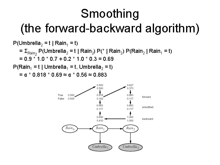
Smoothing (the forward-backward algorithm) P(Umbrella 2 = t | Rain 1 = t) = ΣRain 2 P(Umbrella 2 = t | Rain 2) P(* | Rain 2) P(Rain 2 | Rain 1 = t) = 0. 9 * 1. 0 * 0. 7 + 0. 2 * 1. 0 * 0. 3 = 0. 69 P(Rain 1 = t | Umbrella 1 = t, Umbrella 2 = t) = α * 0. 818 * 0. 69 ≈ α * 0. 56 ≈ 0. 883

Most Likely Explanation (the Viterbi algorithm) P(Rain 1 = t, Rain 2 = t | Umbrella 1 = t, Umbrella 2 = t) = P(Umbrella 1 = t | Rain 1 = t) * P(Rain 2 = t | Rain 1 = t) * P (Umbrella 2 = t | Rain 2 = t) = 0. 818 * 0. 70 * 0. 90 ≈ 0. 515

Speech Recognition (signal preprocessing)

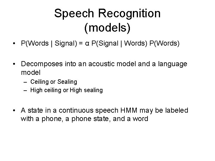
Speech Recognition (models) • P(Words | Signal) = α P(Signal | Words) P(Words) • Decomposes into an acoustic model and a language model – Ceiling or Sealing – High ceiling or High sealing • A state in a continuous speech HMM may be labeled with a phone, a phone state, and a word

Speech Recognition (phones) • Human languages use a limited repertoire of sounds

Speech Recognition (phone model) • Acoustic signal for [t] – Silent beginning – Small explosion in the middle – (Usually) Hissing at the end

Speech Recognition (pronounciation model) • Coarticulation and dialect variations

Speech Recognition (language model) • Can be as simple as bigrams P(Wordi | Word 1: i-1) = P(Wordi | Wordi-1)

References • Artificial Intelligence: A Modern Approach – Second Edition (2003) – Stuart Russell & Peter Norvig • Hidden Markov Model Toolkit (HTK) – http: //htk. eng. cam. ac. uk/ – Nice tutorial (from data prep to evaluation)