Intro to Artificial Intelligence CS 171 Reasoning Under

Intro to Artificial Intelligence CS 171 Reasoning Under Uncertainty Chapter 13 and 14. 1 -14. 2 Andrew Gelfand 3/1/2011

Today… q Representing uncertainty is useful in knowledge bases o Probability provides a coherent framework for uncertainty q Review basic concepts in probability o Emphasis on conditional probability and conditional independence q Full joint distributions are difficult to work with o Conditional independence assumptions allow us to model real-world phenomena with much simpler models q Bayesian networks are a systematic way to build structured distributions q Reading: Chapter 13; beginning of Chapter 14

History of Probability in AI q Early AI (1950’s and 1960’s) o Attempts to solve AI problems using probability met with mixed success q Logical AI (1970’s, 80’s) o Recognized that working with full probability models is intractable o Abandoned probabilistic approaches o Focused on logic-based representations q Probabilistic AI (1990’s-present) o Judea Pearl invents Bayesian networks in 1988 o Realization that working w/ approximate probability models is tractable and useful o Development of machine learning techniques to learn such models from data o Probabilistic techniques now widely used in vision, speech recognition, robotics, language modeling, game-playing, etc

Uncertainty Let action At = leave for airport t minutes before flight Will At get me there on time? Problems: 1. 2. 3. 4. partial observability (road state, other drivers' plans, etc. ) noisy sensors (traffic reports) uncertainty in action outcomes (flat tire, etc. ) immense complexity of modeling and predicting traffic Hence a purely logical approach either 1. 2. risks falsehood: “A 25 will get me there on time”, or leads to conclusions that are too weak for decision making: “A 25 will get me there on time if there's no accident on the bridge and it doesn't rain and my tires remain intact etc. ” (A 1440 might reasonably be said to get me there on time but I'd have to stay overnight in the airport …)

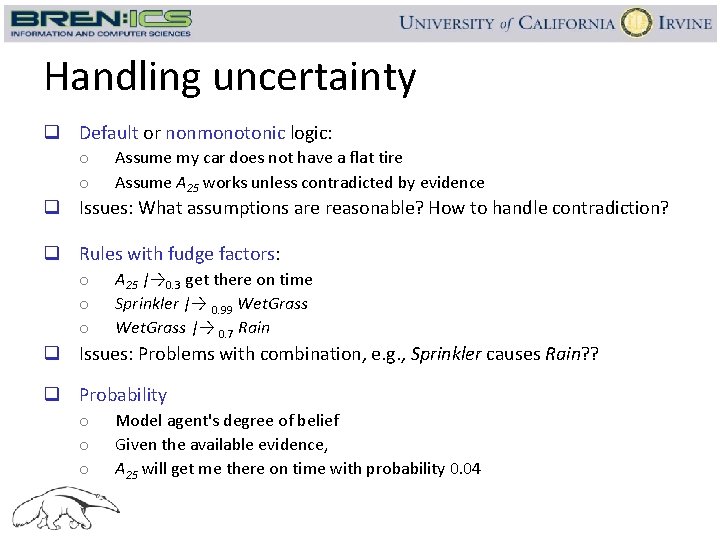
Handling uncertainty q Default or nonmonotonic logic: o o Assume my car does not have a flat tire Assume A 25 works unless contradicted by evidence q Issues: What assumptions are reasonable? How to handle contradiction? q Rules with fudge factors: o o o A 25 |→ 0. 3 get there on time Sprinkler |→ 0. 99 Wet. Grass |→ 0. 7 Rain q Issues: Problems with combination, e. g. , Sprinkler causes Rain? ? q Probability o o o Model agent's degree of belief Given the available evidence, A 25 will get me there on time with probability 0. 04

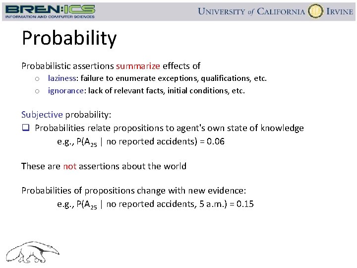
Probability Probabilistic assertions summarize effects of o laziness: failure to enumerate exceptions, qualifications, etc. o ignorance: lack of relevant facts, initial conditions, etc. Subjective probability: q Probabilities relate propositions to agent's own state of knowledge e. g. , P(A 25 | no reported accidents) = 0. 06 These are not assertions about the world Probabilities of propositions change with new evidence: e. g. , P(A 25 | no reported accidents, 5 a. m. ) = 0. 15

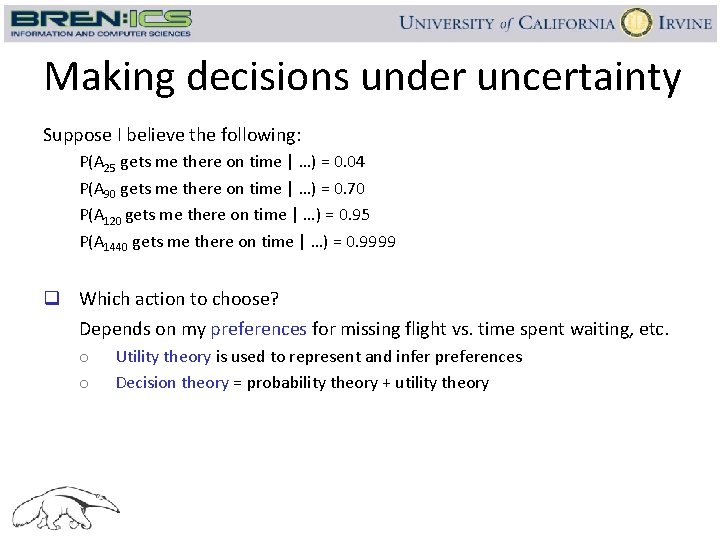
Making decisions under uncertainty Suppose I believe the following: P(A 25 gets me there on time | …) = 0. 04 P(A 90 gets me there on time | …) = 0. 70 P(A 120 gets me there on time | …) = 0. 95 P(A 1440 gets me there on time | …) = 0. 9999 q Which action to choose? Depends on my preferences for missing flight vs. time spent waiting, etc. o o Utility theory is used to represent and infer preferences Decision theory = probability theory + utility theory

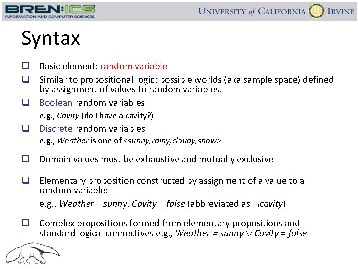
Syntax q Basic element: random variable q Similar to propositional logic: possible worlds (aka sample space) defined by assignment of values to random variables. q Boolean random variables e. g. , Cavity (do I have a cavity? ) q Discrete random variables e. g. , Weather is one of <sunny, rainy, cloudy, snow> q Domain values must be exhaustive and mutually exclusive q Elementary proposition constructed by assignment of a value to a random variable: e. g. , Weather = sunny, Cavity = false (abbreviated as cavity) q Complex propositions formed from elementary propositions and standard logical connectives e. g. , Weather = sunny Cavity = false

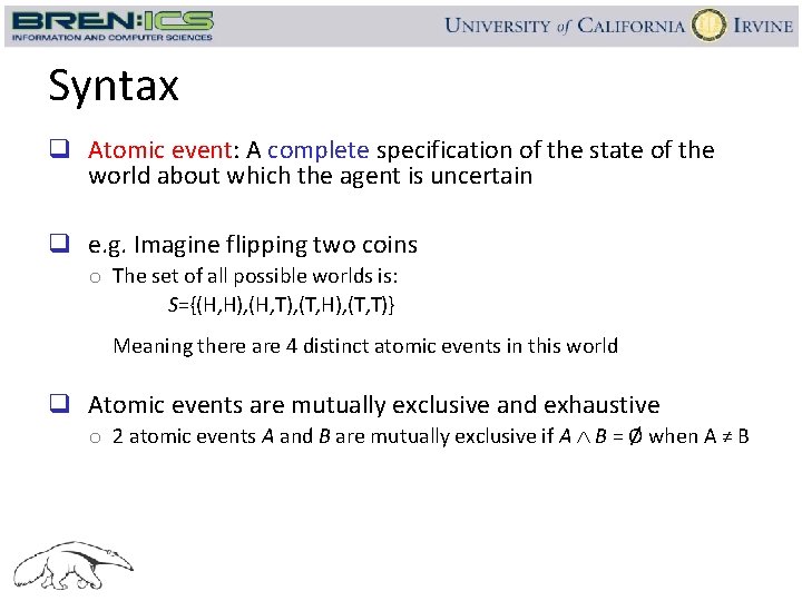
Syntax q Atomic event: A complete specification of the state of the world about which the agent is uncertain q e. g. Imagine flipping two coins o The set of all possible worlds is: S={(H, H), (H, T), (T, H), (T, T)} Meaning there are 4 distinct atomic events in this world q Atomic events are mutually exclusive and exhaustive o 2 atomic events A and B are mutually exclusive if A B = Ø when A ≠ B

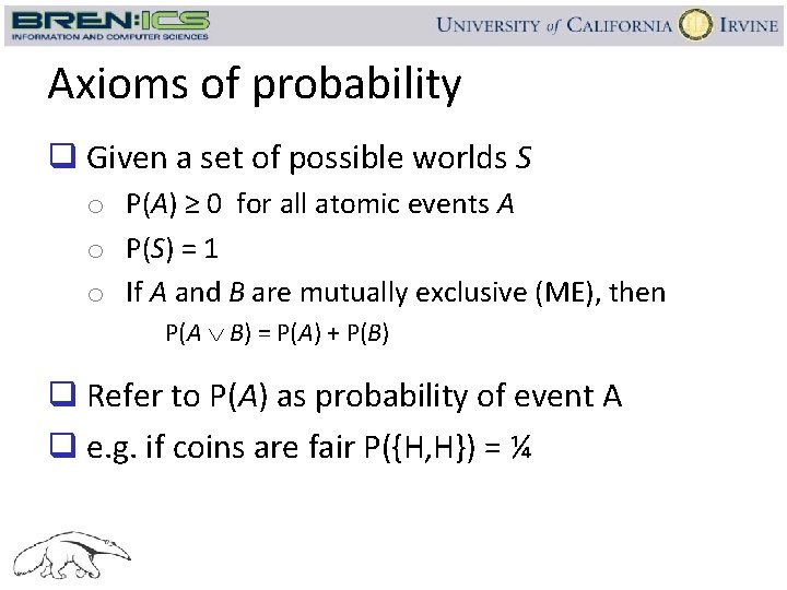
Axioms of probability q Given a set of possible worlds S o P(A) ≥ 0 for all atomic events A o P(S) = 1 o If A and B are mutually exclusive (ME), then P(A B) = P(A) + P(B) q Refer to P(A) as probability of event A q e. g. if coins are fair P({H, H}) = ¼

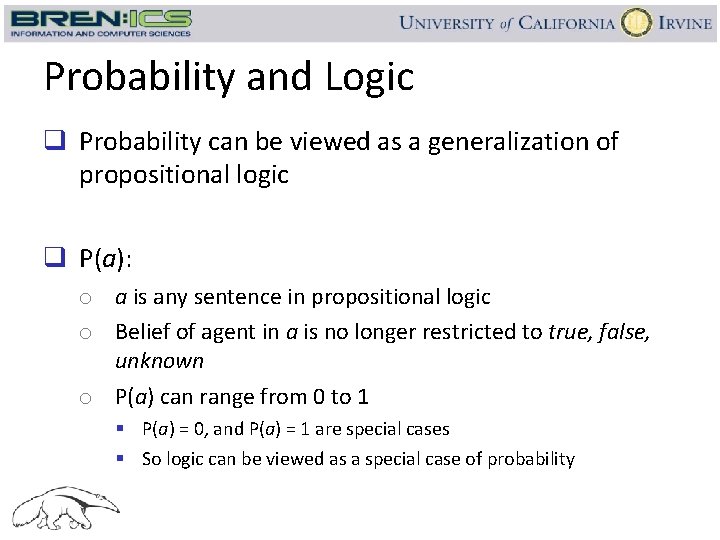
Probability and Logic q Probability can be viewed as a generalization of propositional logic q P(a): o a is any sentence in propositional logic o Belief of agent in a is no longer restricted to true, false, unknown o P(a) can range from 0 to 1 § P(a) = 0, and P(a) = 1 are special cases § So logic can be viewed as a special case of probability

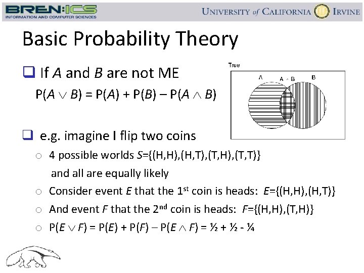
Basic Probability Theory q If A and B are not ME P(A B) = P(A) + P(B) – P(A B) q e. g. imagine I flip two coins o 4 possible worlds S={(H, H), (H, T), (T, H), (T, T)} and all are equally likely o Consider event E that the 1 st coin is heads: E={(H, H), (H, T)} o And event F that the 2 nd coin is heads: F={(H, H), (T, H)} o P(E F) = P(E) + P(F) – P(E F) = ½ + ½ - ¼

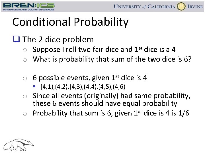
Conditional Probability q The 2 dice problem o Suppose I roll two fair dice and 1 st dice is a 4 o What is probability that sum of the two dice is 6? o 6 possible events, given 1 st dice is 4 § (4, 1), (4, 2), (4, 3), (4, 4), (4, 5), (4, 6) o Since all events (originally) had same probability, these 6 events should have equal probability o Probability that sum is 6, given 1 st dice is 4 is 1/6

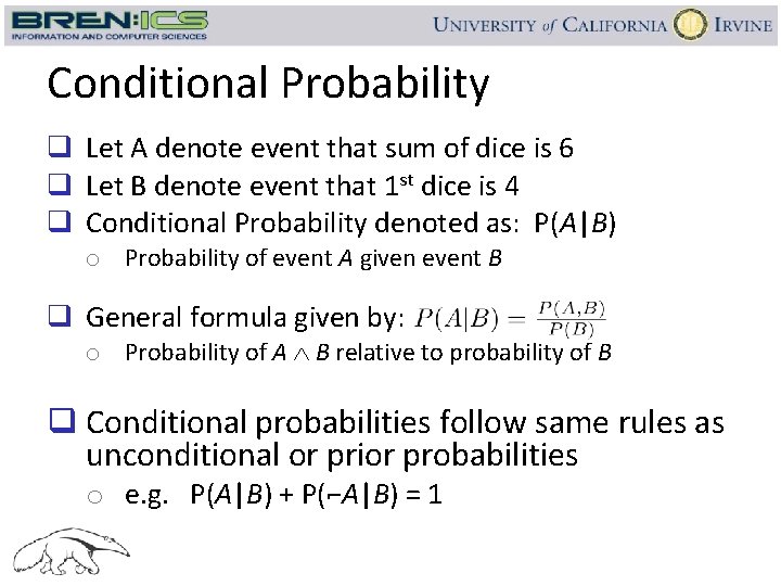
Conditional Probability q Let A denote event that sum of dice is 6 q Let B denote event that 1 st dice is 4 q Conditional Probability denoted as: P(A|B) o Probability of event A given event B q General formula given by: o Probability of A B relative to probability of B q Conditional probabilities follow same rules as unconditional or prior probabilities o e. g. P(A|B) + P(⌐A|B) = 1

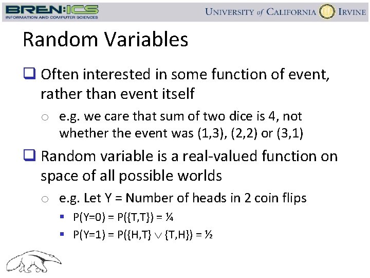
Random Variables q Often interested in some function of event, rather than event itself o e. g. we care that sum of two dice is 4, not whether the event was (1, 3), (2, 2) or (3, 1) q Random variable is a real-valued function on space of all possible worlds o e. g. Let Y = Number of heads in 2 coin flips § P(Y=0) = P({T, T}) = ¼ § P(Y=1) = P({H, T} {T, H}) = ½

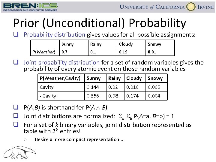
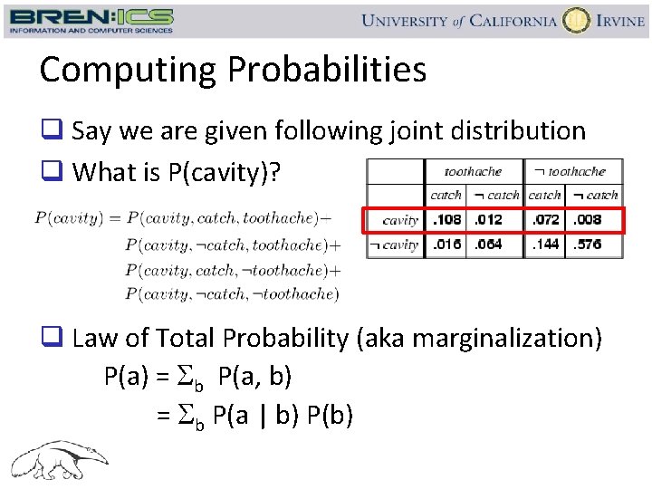
Prior (Unconditional) Probability q Probability distribution gives values for all possible assignments: P(Weather) Sunny Rainy Cloudy Snowy 0. 7 0. 19 0. 01 q Joint probability distribution for a set of random variables gives the probability of every atomic event on those random variables P(Weather, Cavity) Sunny Rainy Cloudy Snowy Cavity 0. 144 0. 02 0. 016 0. 006 ⌐Cavity 0. 556 0. 08 0. 174 0. 004 q P(A, B) is shorthand for P(A B) q Joint distributions are normalized: Sa Sb P(A=a, B=b) = 1 q For a set of k binary variables, joint distribution represented as table with 2 k entries! o Desire a more compact representation…

Computing Probabilities q Say we are given following joint distribution q What is P(cavity)? q Law of Total Probability (aka marginalization) P(a) = Sb P(a, b) = Sb P(a | b) P(b)

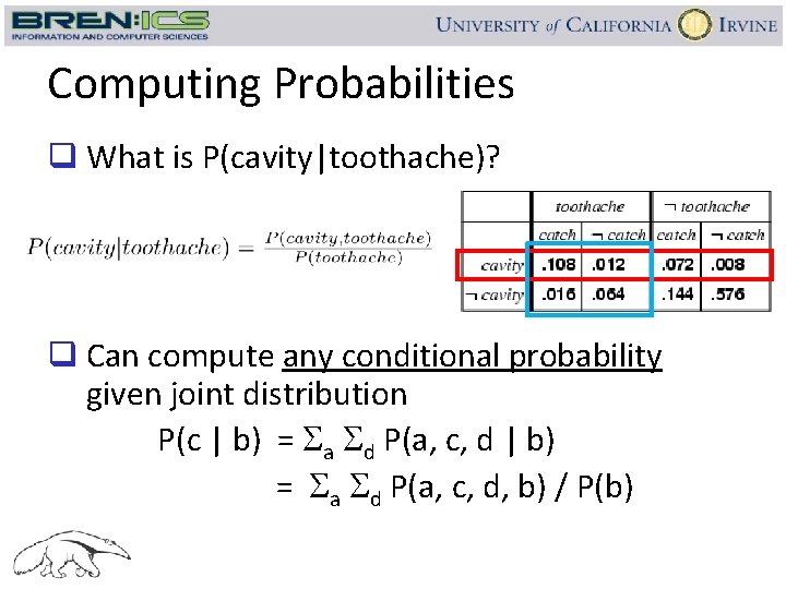
Computing Probabilities q What is P(cavity|toothache)? q Can compute any conditional probability given joint distribution P(c | b) = Sa Sd P(a, c, d, b) / P(b)

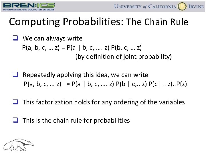
Computing Probabilities: The Chain Rule q We can always write P(a, b, c, … z) = P(a | b, c, …. z) P(b, c, … z) (by definition of joint probability) q Repeatedly applying this idea, we can write P(a, b, c, … z) = P(a | b, c, …. z) P(b | c, . . z) P(c|. . z). . P(z) q This factorization holds for any ordering of the variables q This is the chain rule for probabilities

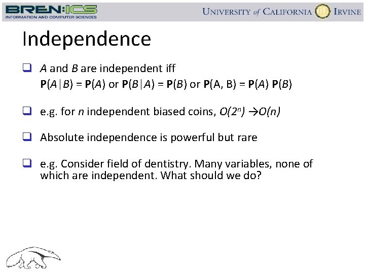
Independence q A and B are independent iff P(A|B) = P(A) or P(B|A) = P(B) or P(A, B) = P(A) P(B) q e. g. for n independent biased coins, O(2 n) →O(n) q Absolute independence is powerful but rare q e. g. Consider field of dentistry. Many variables, none of which are independent. What should we do?

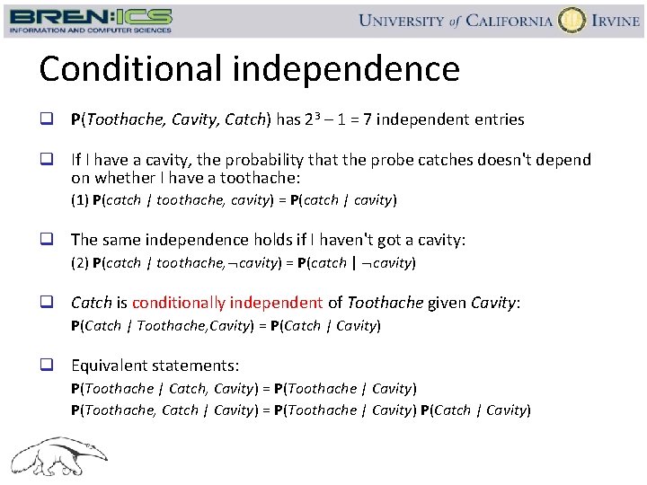
Conditional independence q P(Toothache, Cavity, Catch) has 23 – 1 = 7 independent entries q If I have a cavity, the probability that the probe catches doesn't depend on whether I have a toothache: (1) P(catch | toothache, cavity) = P(catch | cavity) q The same independence holds if I haven't got a cavity: (2) P(catch | toothache, cavity) = P(catch | cavity) q Catch is conditionally independent of Toothache given Cavity: P(Catch | Toothache, Cavity) = P(Catch | Cavity) q Equivalent statements: P(Toothache | Catch, Cavity) = P(Toothache | Cavity) P(Toothache, Catch | Cavity) = P(Toothache | Cavity) P(Catch | Cavity)

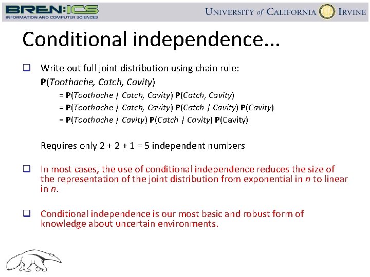
Conditional independence. . . q Write out full joint distribution using chain rule: P(Toothache, Catch, Cavity) = P(Toothache | Catch, Cavity) P(Catch | Cavity) P(Cavity) = P(Toothache | Cavity) P(Catch | Cavity) P(Cavity) Requires only 2 + 1 = 5 independent numbers q In most cases, the use of conditional independence reduces the size of the representation of the joint distribution from exponential in n to linear in n. q Conditional independence is our most basic and robust form of knowledge about uncertain environments.

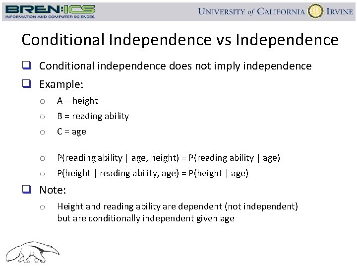
Conditional Independence vs Independence q Conditional independence does not imply independence q Example: o A = height o B = reading ability o C = age o P(reading ability | age, height) = P(reading ability | age) o P(height | reading ability, age) = P(height | age) q Note: o Height and reading ability are dependent (not independent) but are conditionally independent given age

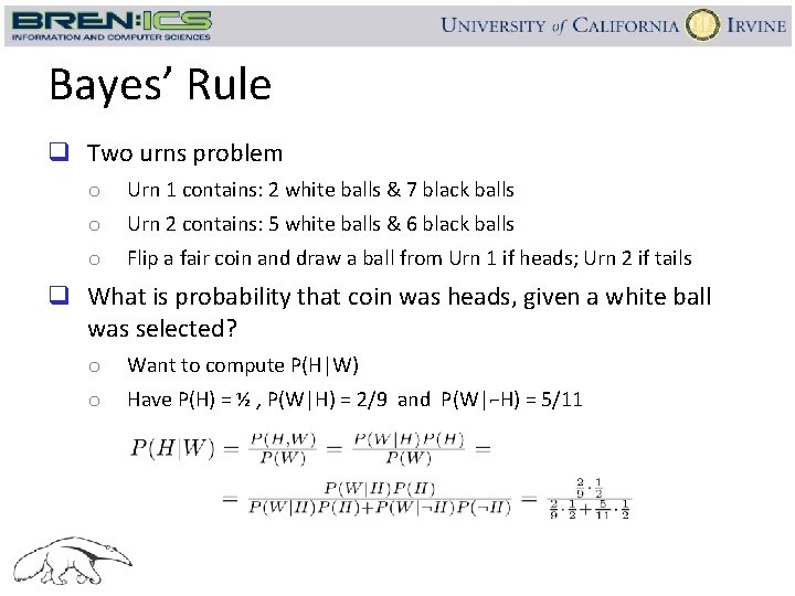
Bayes’ Rule q Two urns problem o Urn 1 contains: 2 white balls & 7 black balls o Urn 2 contains: 5 white balls & 6 black balls o Flip a fair coin and draw a ball from Urn 1 if heads; Urn 2 if tails q What is probability that coin was heads, given a white ball was selected? o Want to compute P(H|W) o Have P(H) = ½ , P(W|H) = 2/9 and P(W|⌐H) = 5/11

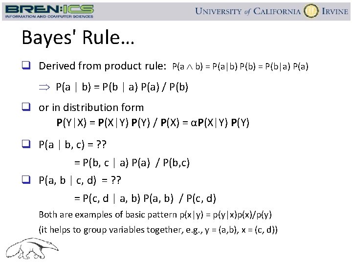
Bayes' Rule… q Derived from product rule: P(a b) = P(a|b) P(b) = P(b|a) P(a) P(a | b) = P(b | a) P(a) / P(b) q or in distribution form P(Y|X) = P(X|Y) P(Y) / P(X) = αP(X|Y) P(Y) q P(a | b, c) = ? ? = P(b, c | a) P(a) / P(b, c) q P(a, b | c, d) = ? ? = P(c, d | a, b) P(a, b) / P(c, d) Both are examples of basic pattern p(x|y) = p(y|x)p(x)/p(y) (it helps to group variables together, e. g. , y = (a, b), x = (c, d))

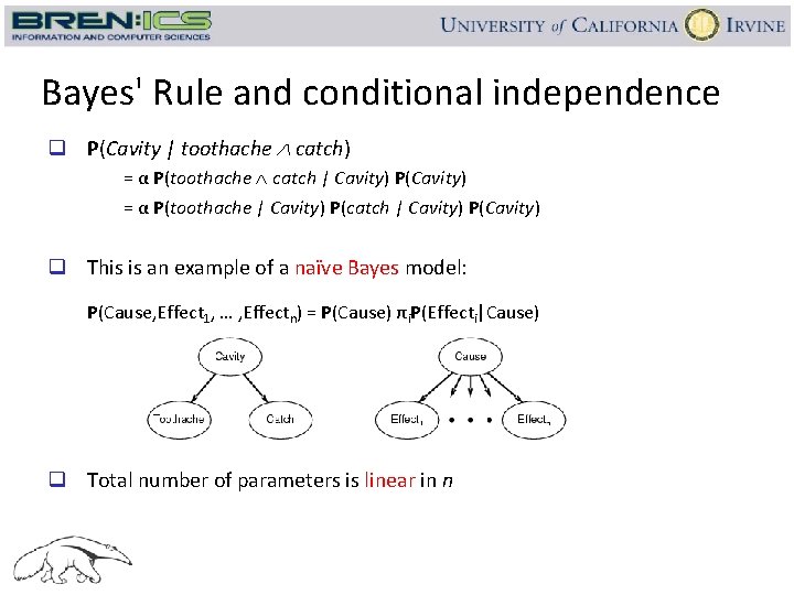
Bayes' Rule and conditional independence q P(Cavity | toothache catch) = α P(toothache catch | Cavity) P(Cavity) = α P(toothache | Cavity) P(catch | Cavity) P(Cavity) q This is an example of a naïve Bayes model: P(Cause, Effect 1, … , Effectn) = P(Cause) πi. P(Effecti|Cause) q Total number of parameters is linear in n

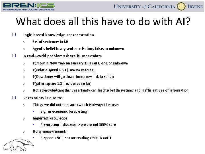
What does all this have to do with AI? q q q Logic-based knowledge representation o Set of sentences in KB o Agent’s belief in any sentence is: true, false, or unknown In real-world problems there is uncertainty o P(snow in New York on January 1) is not 0 or 1 or unknown o P(vehicle speed > 50 | sensor reading) o P(Dow Jones will go down tomorrow | data so far) o P(pit in square 2, 2 | evidence so far) o Not acknowledging this uncertainty can lead to brittle systems and inefficient use of information Uncertainty is due to: o Things we did not measure (which is always the case) § o Imperfect knowledge § o E. g. , in economic forecasting P(symptom | disease) -> we are not 100% sure Noisy measurements § P(speed > 50 | sensor reading > 50) is not 1

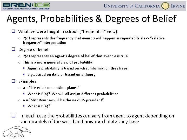
Agents, Probabilities & Degrees of Belief q What we were taught in school (“frequentist” view) o P(a) represents the frequency that event a will happen in repeated trials -> “relative frequency” interpretation q Degree of belief o P(a) represents an agent’s degree of belief that event a is true o This is a more general view of probability § Agent’s probability is based on what information they have § E. g. , based on data or based on a theory q Examples: o a = “life exists on another planet” § What is P(a)? We will assign different probabilities o a = “Mitt Romney will be the next US president” § What is P(a)? q In each case the probabilities can vary from agent to agent depending on their models of the world and how much data they have

More on Degrees of Belief q Our interpretation of P(a | e) is that it is an agent’s degree of belief in the proposition a, given evidence e o Note that proposition a is true or false in the real-world o P(a|e) reflects the agent’s uncertainty or ignorance q The degree of belief interpretation does not mean that we need new or different rules for working with probabilities o The same rules (Bayes rule, law of total probability, probabilities sum to 1) still apply – our interpretation is different q If Agent 1 has inconsistent sets of probabilities (violate axioms of probability theory) then there exists a betting strategy that allows Agent 2 to always win in bets against Agent 1 o See de Finetti’s argument in the text

Maximizing expected utility q What action should the agent take? o A rational agent should maximize expected utility, or equivalently minimize expected cost q Expected cost of actions: E[ cost(a) ] = 30 p(c) – 50 [1 – p(c) ] E[ cost(b) ] = -100 p(c) Break even point? 30 p – 50 + 50 p = -100 p + 30 p + 50 p = 50 => p(c) = 50/180 ~ 0. 28 If p(c) > 0. 28, the optimal decision is to operate q Original theory from economics, cognitive science (1950’s) - But widely used in modern AI, e. g. , in robotics, vision, game-playing q Can only make optimal decisions if know the probabilities

Constructing a Propositional Probabilistic Knowledge Base q Define all variables of interest: A, B, C, … Z q Define a joint probability table for P(A, B, C, … Z) o We have seen earlier how this will allow us to compute the answer to any query, p(query | evidence), where query and evidence = any propositional sentence q 2 major problems: o Computation time: § o Model specification § o P(a|b) requires summing out over all other variables in the model, e. g. , O(m. K-1) with K variables Joint table has O(m. K) entries – where will all the numbers come from? These 2 problems effectively halted the use of probability in AI research from the 1960’s up until about 1990

Bayesian Networks

A Whodunit q You return home from a long day to find that your house guest has been murdered. o There are two culprits: 1) The Butler; and 2) The Cook o There are three possible weapons: 1) A knife; 2) A gun; and 3) A candlestick q Lets use probabilistic reasoning to find out whodunit?

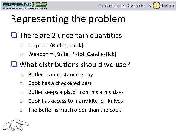
Representing the problem q There are 2 uncertain quantities o Culprit = {Butler, Cook} o Weapon = {Knife, Pistol, Candlestick} q What distributions should we use? o o o Butler is an upstanding guy Cook has a checkered past Butler keeps a pistol from his army days Cook has access to many kitchen knives The Butler is much older than the cook

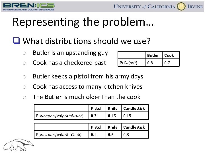
Representing the problem… q What distributions should we use? o Butler is an upstanding guy o Cook has a checkered past P(Culprit) o Butler keeps a pistol from his army days o Cook has access to many kitchen knives o The Butler is much older than the cook P(weapon|culprit=Butler) P(weapon|culprit=Cook) Pistol Knife Candlestick 0. 7 0. 15 Pistol Knife Candlestick 0. 1 0. 6 0. 3 Butler Cook 0. 3 0. 7

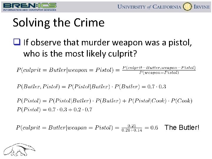
Solving the Crime q If observe that murder weapon was a pistol, who is the most likely culprit? The Butler!

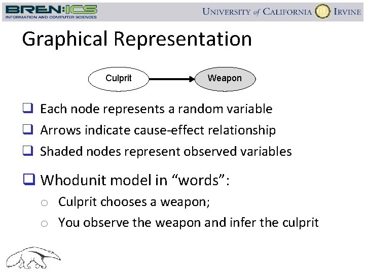
Graphical Representation Culprit Weapon q Each node represents a random variable q Arrows indicate cause-effect relationship q Shaded nodes represent observed variables q Whodunit model in “words”: o Culprit chooses a weapon; o You observe the weapon and infer the culprit

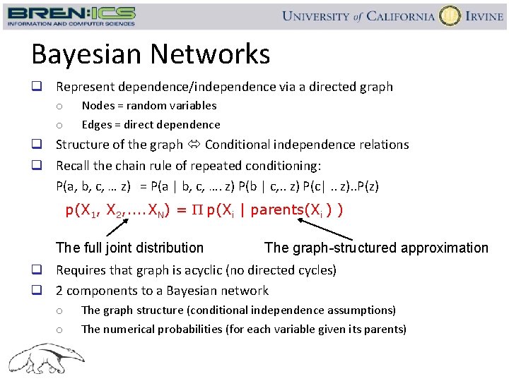
Bayesian Networks q Represent dependence/independence via a directed graph o o Nodes = random variables Edges = direct dependence q Structure of the graph Conditional independence relations q Recall the chain rule of repeated conditioning: P(a, b, c, … z) = P(a | b, c, …. z) P(b | c, . . z) P(c|. . z). . P(z) p(X 1, X 2, . . XN) = p(Xi | parents(Xi ) ) The full joint distribution The graph-structured approximation q Requires that graph is acyclic (no directed cycles) q 2 components to a Bayesian network o o The graph structure (conditional independence assumptions) The numerical probabilities (for each variable given its parents)

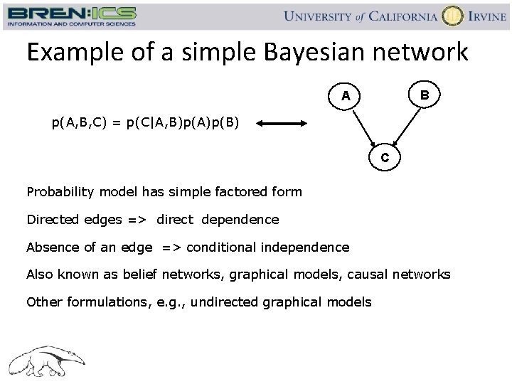
Example of a simple Bayesian network B A p(A, B, C) = p(C|A, B)p(A)p(B) C Probability model has simple factored form Directed edges => direct dependence Absence of an edge => conditional independence Also known as belief networks, graphical models, causal networks Other formulations, e. g. , undirected graphical models

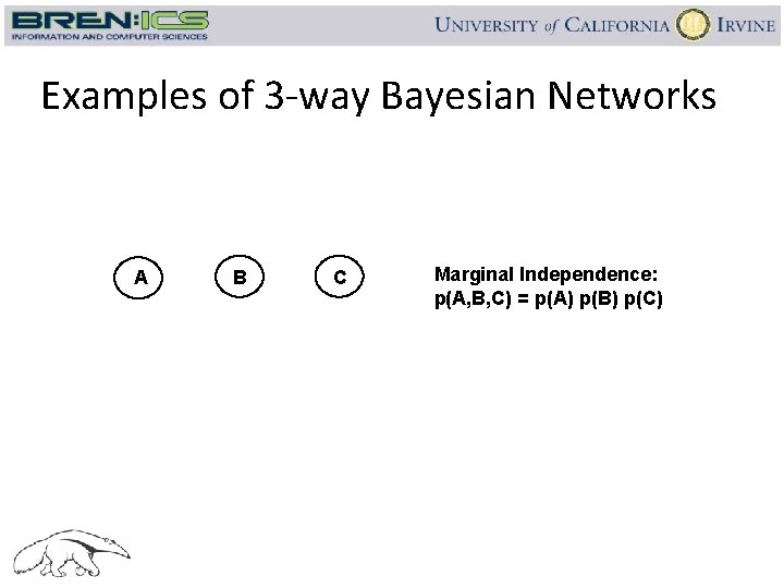
Examples of 3 -way Bayesian Networks A B C Marginal Independence: p(A, B, C) = p(A) p(B) p(C)

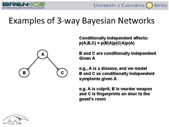
Examples of 3 -way Bayesian Networks Conditionally independent effects: p(A, B, C) = p(B|A)p(C|A)p(A) B and C are conditionally independent Given A A B C e. g. , A is a disease, and we model B and C as conditionally independent symptoms given A e. g. A is culprit, B is murder weapon and C is fingerprints on door to the guest’s room

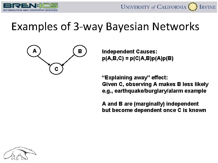
Examples of 3 -way Bayesian Networks A B Independent Causes: p(A, B, C) = p(C|A, B)p(A)p(B) C “Explaining away” effect: Given C, observing A makes B less likely e. g. , earthquake/burglary/alarm example A and B are (marginally) independent but become dependent once C is known

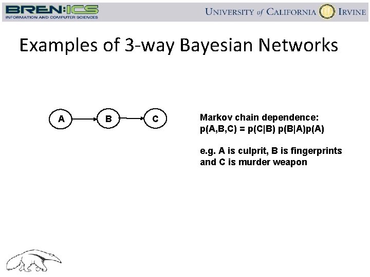
Examples of 3 -way Bayesian Networks A B C Markov chain dependence: p(A, B, C) = p(C|B) p(B|A)p(A) e. g. A is culprit, B is fingerprints and C is murder weapon

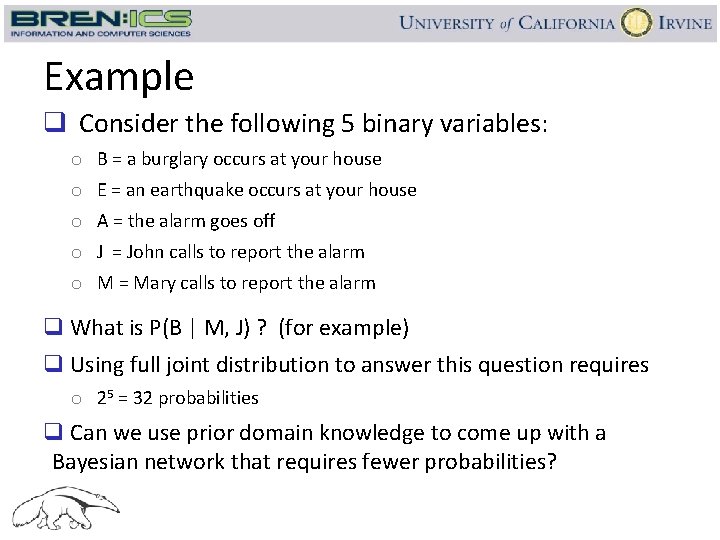
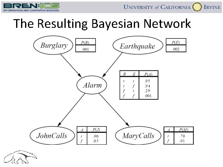
Example q Consider the following 5 binary variables: o B = a burglary occurs at your house o E = an earthquake occurs at your house o A = the alarm goes off o J = John calls to report the alarm o M = Mary calls to report the alarm q What is P(B | M, J) ? (for example) q Using full joint distribution to answer this question requires o 25 = 32 probabilities q Can we use prior domain knowledge to come up with a Bayesian network that requires fewer probabilities?

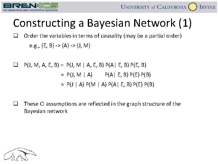
Constructing a Bayesian Network (1) q Order the variables in terms of causality (may be a partial order) e. g. , {E, B} -> {A} -> {J, M} q P(J, M, A, E, B) = P(J, M | A, E, B) P(A| E, B) P(E, B) ≈ P(J, M | A) P(A| E, B) P(E) P(B) ≈ P(J | A) P(M | A) P(A| E, B) P(E) P(B) q These CI assumptions are reflected in the graph structure of the Bayesian network

The Resulting Bayesian Network

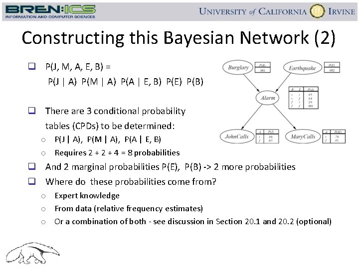
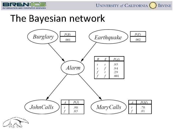
Constructing this Bayesian Network (2) q P(J, M, A, E, B) = P(J | A) P(M | A) P(A | E, B) P(E) P(B) q There are 3 conditional probability tables (CPDs) to be determined: o P(J | A), P(M | A), P(A | E, B) o Requires 2 + 4 = 8 probabilities q And 2 marginal probabilities P(E), P(B) -> 2 more probabilities q Where do these probabilities come from? o Expert knowledge o From data (relative frequency estimates) o Or a combination of both - see discussion in Section 20. 1 and 20. 2 (optional)

The Bayesian network

Number of Probabilities in Bayes Nets q Consider n binary variables q Unconstrained joint distribution requires O(2 n) probabilities q If we have a Bayesian network, with a maximum of k parents for any node, then we need O(n 2 k) probabilities q Example o Full unconstrained joint distribution § o n = 30: need 109 probabilities for full joint distribution Bayesian network § n = 30, k = 4: need 480 probabilities

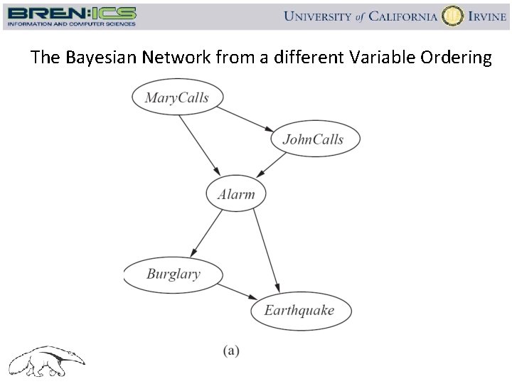
The Bayesian Network from a different Variable Ordering

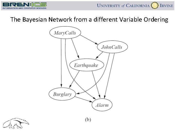
The Bayesian Network from a different Variable Ordering

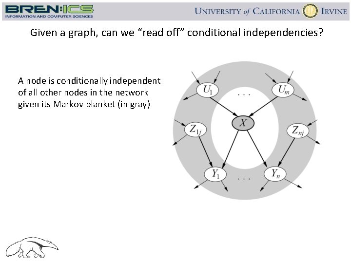
Given a graph, can we “read off” conditional independencies? A node is conditionally independent of all other nodes in the network given its Markov blanket (in gray)

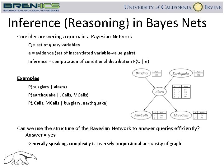
Inference (Reasoning) in Bayes Nets Consider answering a query in a Bayesian Network Q = set of query variables e = evidence (set of instantiated variable-value pairs) Inference = computation of conditional distribution P(Q | e) Examples P(burglary | alarm) P(earthquake | JCalls, MCalls) P(JCalls, MCalls | burglary, earthquake) Can we use the structure of the Bayesian Network to answer queries efficiently? Answer = yes Generally speaking, complexity is inversely proportional to sparsity of graph

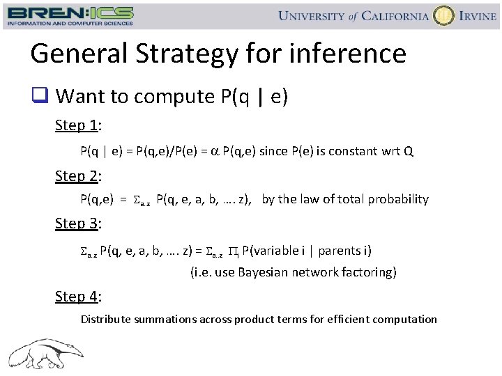
General Strategy for inference q Want to compute P(q | e) Step 1: P(q | e) = P(q, e)/P(e) = a P(q, e) since P(e) is constant wrt Q Step 2: P(q, e) = Sa. . z P(q, e, a, b, …. z), by the law of total probability Step 3: Sa. . z P(q, e, a, b, …. z) = Sa. . z i P(variable i | parents i) (i. e. use Bayesian network factoring) Step 4: Distribute summations across product terms for efficient computation

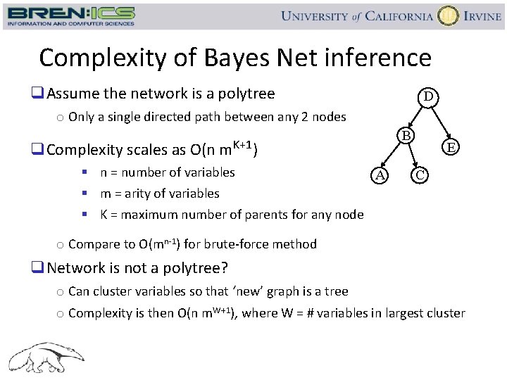
Complexity of Bayes Net inference q. Assume the network is a polytree D o Only a single directed path between any 2 nodes q. Complexity scales as O(n m. K+1) § n = number of variables A § m = arity of variables § K = maximum number of parents for any node B E C o Compare to O(mn-1) for brute-force method q. Network is not a polytree? o Can cluster variables so that ‘new’ graph is a tree o Complexity is then O(n m. W+1), where W = # variables in largest cluster

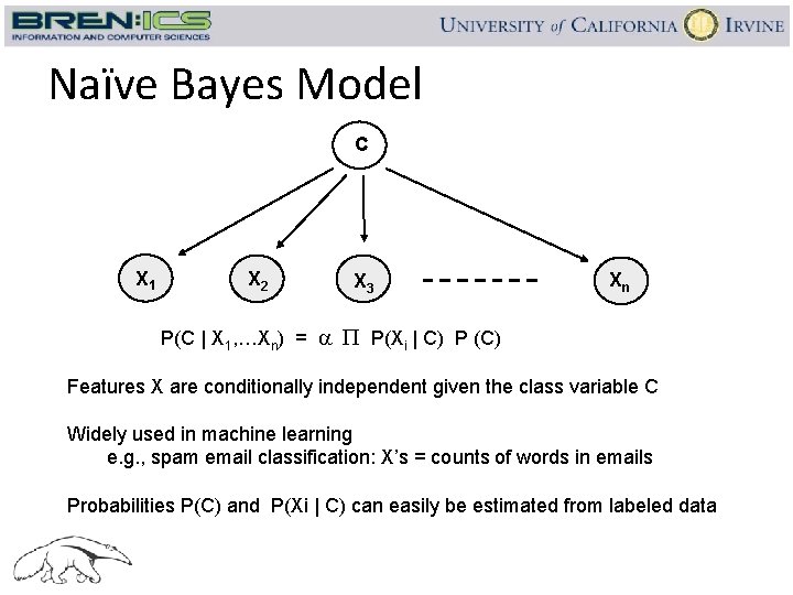
Naïve Bayes Model C X 1 X 2 X 3 Xn P(C | X 1, …Xn) = a P(Xi | C) P (C) Features X are conditionally independent given the class variable C Widely used in machine learning e. g. , spam email classification: X’s = counts of words in emails Probabilities P(C) and P(Xi | C) can easily be estimated from labeled data

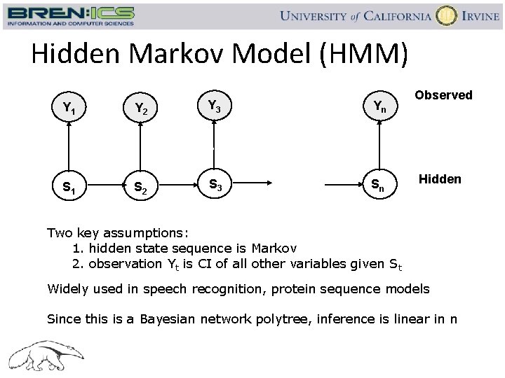
Hidden Markov Model (HMM) Y 1 Y 2 Y 3 Yn Observed --------------------------S 1 S 2 S 3 Sn Hidden Two key assumptions: 1. hidden state sequence is Markov 2. observation Yt is CI of all other variables given St Widely used in speech recognition, protein sequence models Since this is a Bayesian network polytree, inference is linear in n

Summary q Bayesian networks represent joint distributions using a graph q The graph encodes a set of conditional independence assumptions q Answering queries (i. e. inference) in a Bayesian network amounts to efficient computation of appropriate conditional probabilities q Probabilistic inference is intractable in the general case o Can be done in linear time for certain classes of Bayesian networks