CS 4700 Foundations of Artificial Intelligence Bart Selman

CS 4700: Foundations of Artificial Intelligence Bart Selman selman@cs. cornell. edu Informed Search Readings R&N - Chapter 3: 3. 5 and 3. 6
Search strategies determined by choice of node (in queue) to expand Uninformed search: – Distance to goal not taken into account Informed search : – Information about cost to goal taken into account Aside: “Cleverness” about what option to explore next, almost seems a hallmark of intelligence. E. g. , a sense of what might be a good move in chess or what step to try next in a mathematical proof. We don’t do blind search…
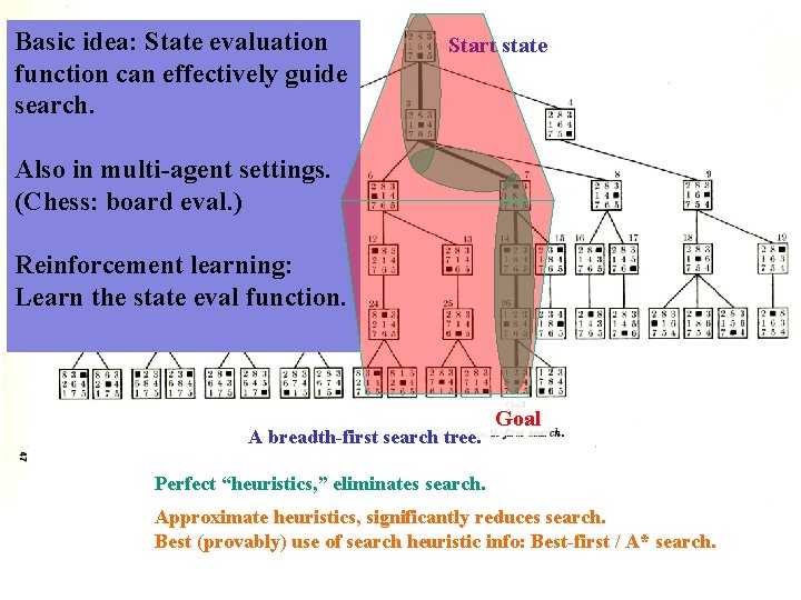
Basic idea: State evaluation function can effectively guide search. Start state Also in multi-agent settings. (Chess: board eval. ) Reinforcement learning: Learn the state eval function. A breadth-first search tree. Goal Perfect “heuristics, ” eliminates search. Approximate heuristics, significantly reduces search. Best (provably) use of search heuristic info: Best-first / A* search.
Outline • • Best-first search Greedy best-first search A* search Heuristics
How to take information into account? Best-first search. Idea : use an evaluation function for each node – Estimate of “desirability” of node – Expand most desirable unexpanded node first (“best-first search”) – Heuristic Functions : • f: States Numbers • f(n): expresses the quality of the state n – Allows us to express problem-specific knowledge, – Can be imported in a generic way in the algorithms. – Use uniform-cost search. See Figure 3. 14 but use f(n) instead of path cost g(n). Note: g(n) = cost so far to reach n – Queuing based on f(n): Order the nodes in fringe in decreasing order of desirability Special cases: • greedy best-first search • A* search
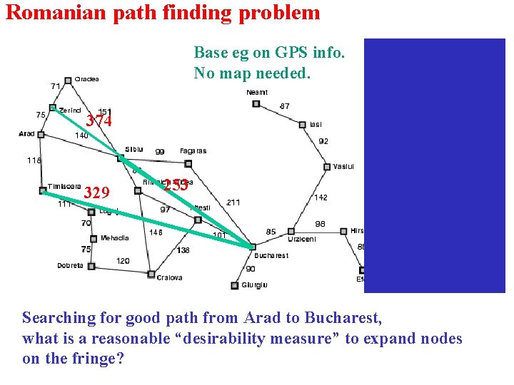
Romanian path finding problem Base eg on GPS info. No map needed. Straight-line dist. to Bucharest 374 329 253 Searching for good path from Arad to Bucharest, what is a reasonable “desirability measure” to expand nodes on the fringe?
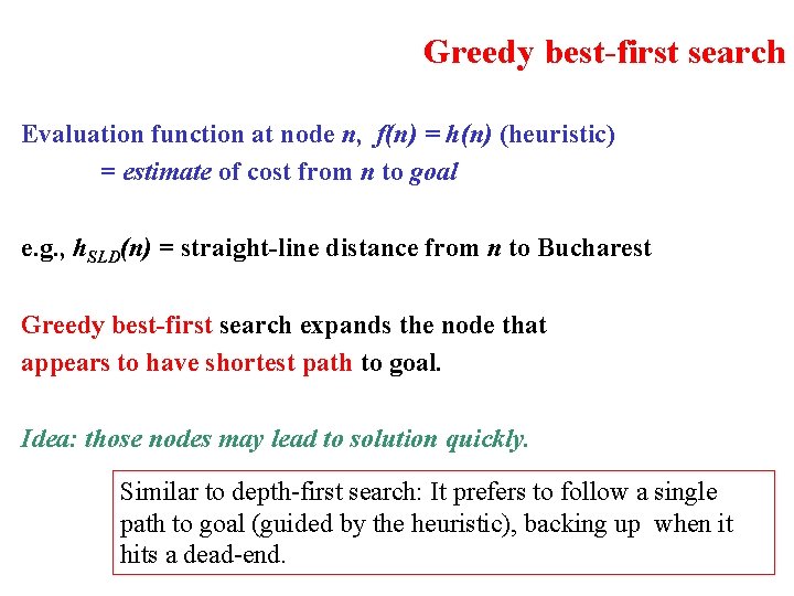
Greedy best-first search Evaluation function at node n, f(n) = h(n) (heuristic) = estimate of cost from n to goal e. g. , h. SLD(n) = straight-line distance from n to Bucharest Greedy best-first search expands the node that appears to have shortest path to goal. Idea: those nodes may lead to solution quickly. Similar to depth-first search: It prefers to follow a single path to goal (guided by the heuristic), backing up when it hits a dead-end.
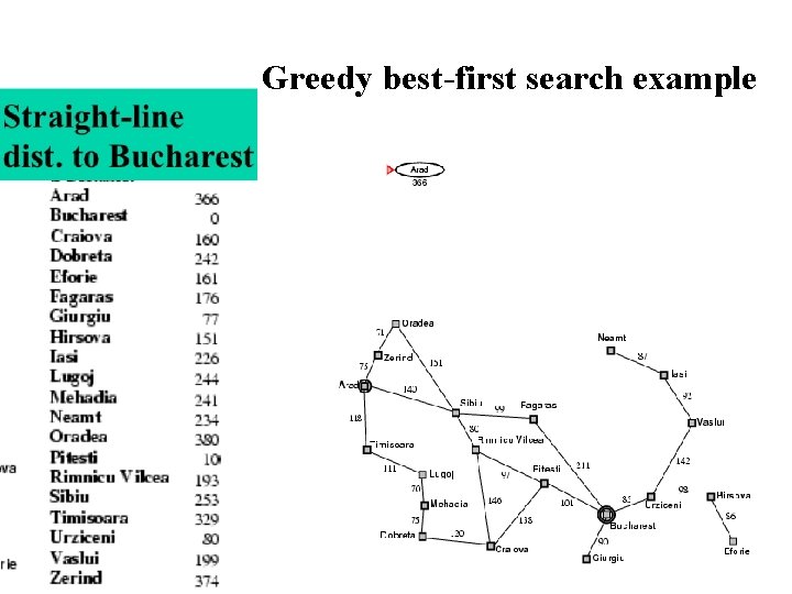
Greedy best-first search example
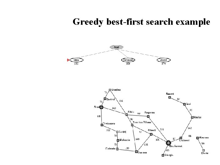
Greedy best-first search example
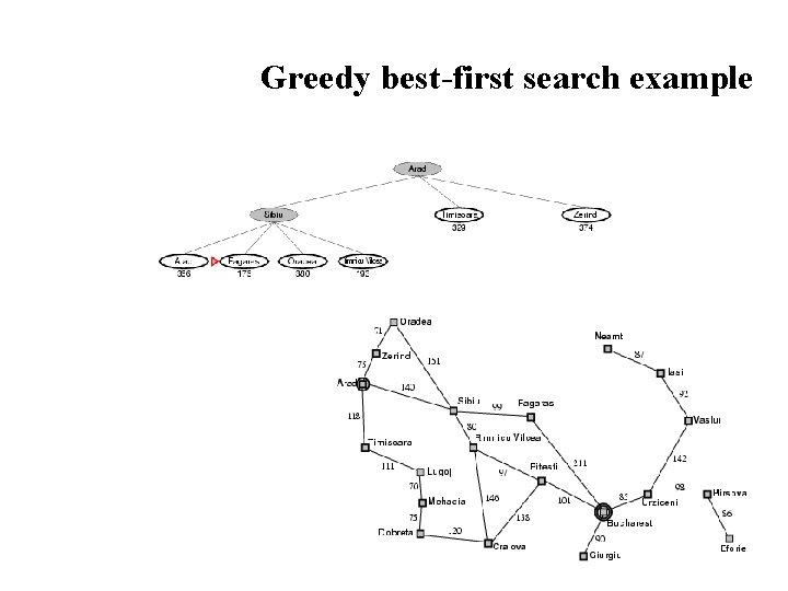
Greedy best-first search example
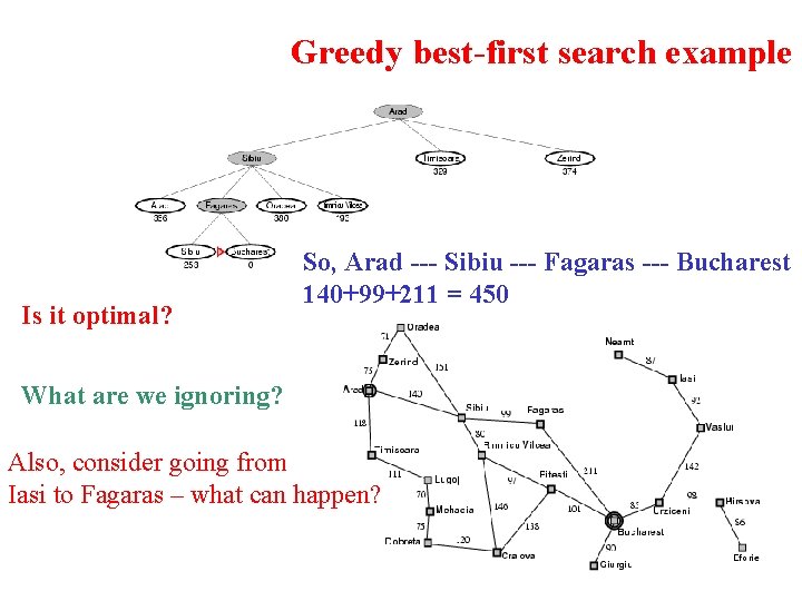
Greedy best-first search example Is it optimal? So, Arad --- Sibiu --- Fagaras --- Bucharest 140+99+211 = 450 What are we ignoring? Also, consider going from Iasi to Fagaras – what can happen?
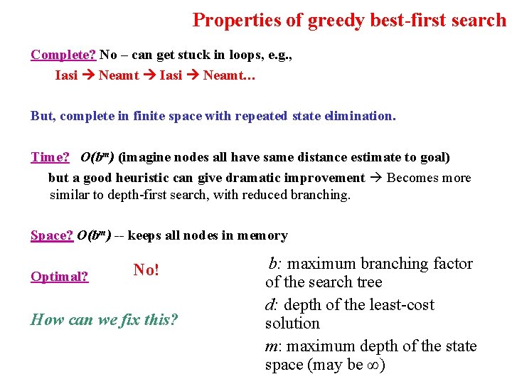
Properties of greedy best-first search Complete? No – can get stuck in loops, e. g. , Iasi Neamt… But, complete in finite space with repeated state elimination. Time? O(bm) (imagine nodes all have same distance estimate to goal) but a good heuristic can give dramatic improvement Becomes more similar to depth-first search, with reduced branching. Space? O(bm) -- keeps all nodes in memory Optimal? No! How can we fix this? b: maximum branching factor of the search tree d: depth of the least-cost solution m: maximum depth of the state space (may be ∞)
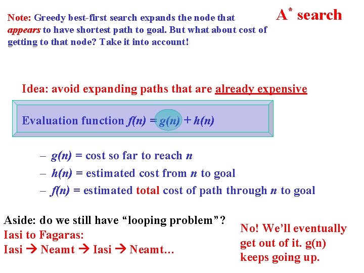
Note: Greedy best-first search expands the node that appears to have shortest path to goal. But what about cost of getting to that node? Take it into account! A* search Idea: avoid expanding paths that are already expensive Evaluation function f(n) = g(n) + h(n) – g(n) = cost so far to reach n – h(n) = estimated cost from n to goal – f(n) = estimated total cost of path through n to goal Aside: do we still have “looping problem”? Iasi to Fagaras: Iasi Neamt… No! We’ll eventually get out of it. g(n) keeps going up.
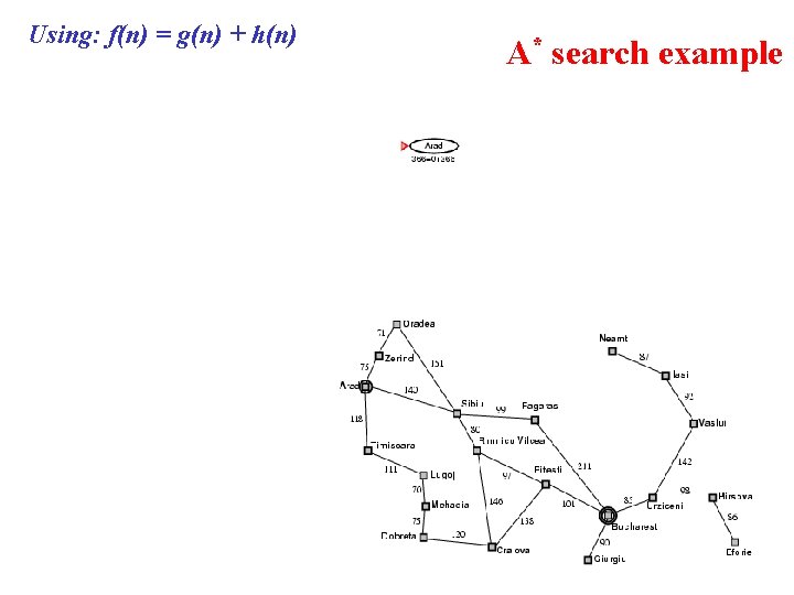
Using: f(n) = g(n) + h(n) A* search example
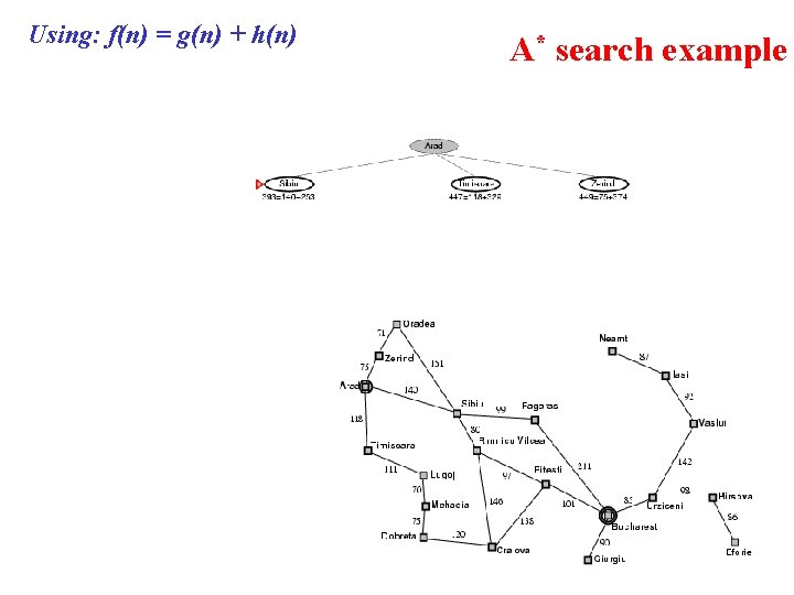
Using: f(n) = g(n) + h(n) A* search example
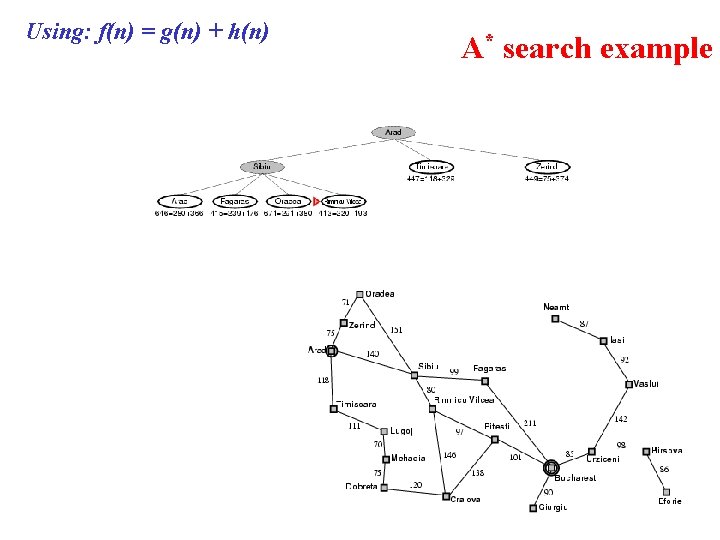
Using: f(n) = g(n) + h(n) A* search example
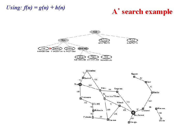
Using: f(n) = g(n) + h(n) A* search example
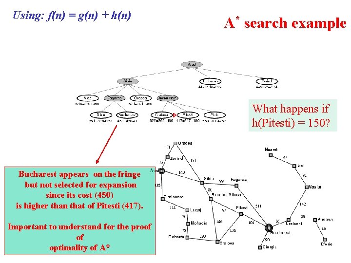
Using: f(n) = g(n) + h(n) A* search example What happens if h(Pitesti) = 150? Bucharest appears on the fringe but not selected for expansion since its cost (450) is higher than that of Pitesti (417). Important to understand for the proof of optimality of A*
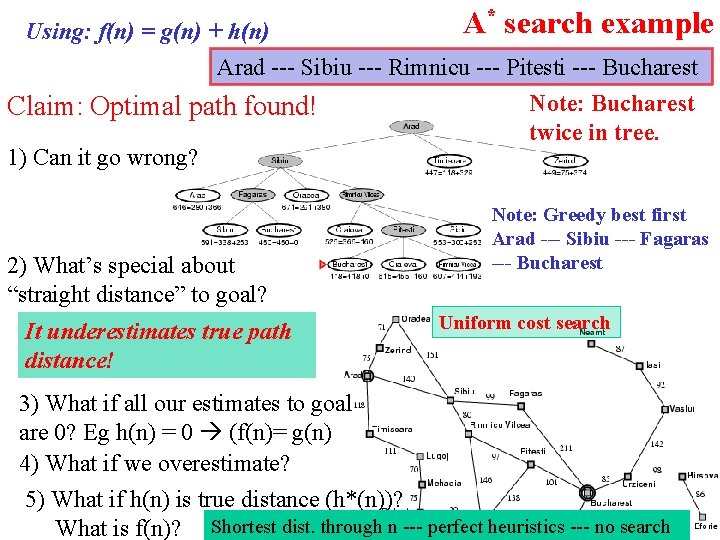
A* search example Using: f(n) = g(n) + h(n) Arad --- Sibiu --- Rimnicu --- Pitesti --- Bucharest Note: Bucharest Claim: Optimal path found! twice in tree. 1) Can it go wrong? 2) What’s special about “straight distance” to goal? It underestimates true path distance! Note: Greedy best first Arad --- Sibiu --- Fagaras --- Bucharest Uniform cost search 3) What if all our estimates to goal are 0? Eg h(n) = 0 (f(n)= g(n) 4) What if we overestimate? 5) What if h(n) is true distance (h*(n))? What is f(n)? Shortest dist. through n --- perfect heuristics --- no search
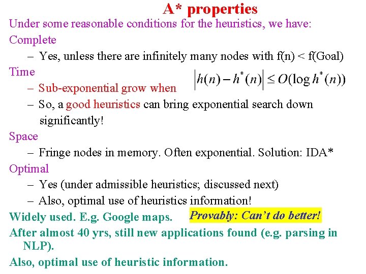
A* properties Under some reasonable conditions for the heuristics, we have: Complete – Yes, unless there are infinitely many nodes with f(n) < f(Goal) Time – Sub-exponential grow when – So, a good heuristics can bring exponential search down significantly! Space – Fringe nodes in memory. Often exponential. Solution: IDA* Optimal – Yes (under admissible heuristics; discussed next) – Also, optimal use of heuristics information! Widely used. E. g. Google maps. Provably: Can’t do better! After almost 40 yrs, still new applications found (e. g. parsing in NLP). Also, optimal use of heuristic information.
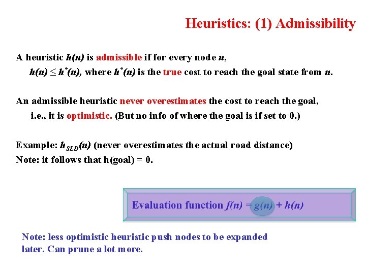
Heuristics: (1) Admissibility A heuristic h(n) is admissible if for every node n, h(n) ≤ h*(n), where h*(n) is the true cost to reach the goal state from n. An admissible heuristic never overestimates the cost to reach the goal, i. e. , it is optimistic. (But no info of where the goal is if set to 0. ) Example: h. SLD(n) (never overestimates the actual road distance) Note: it follows that h(goal) = 0. Note: less optimistic heuristic push nodes to be expanded later. Can prune a lot more.
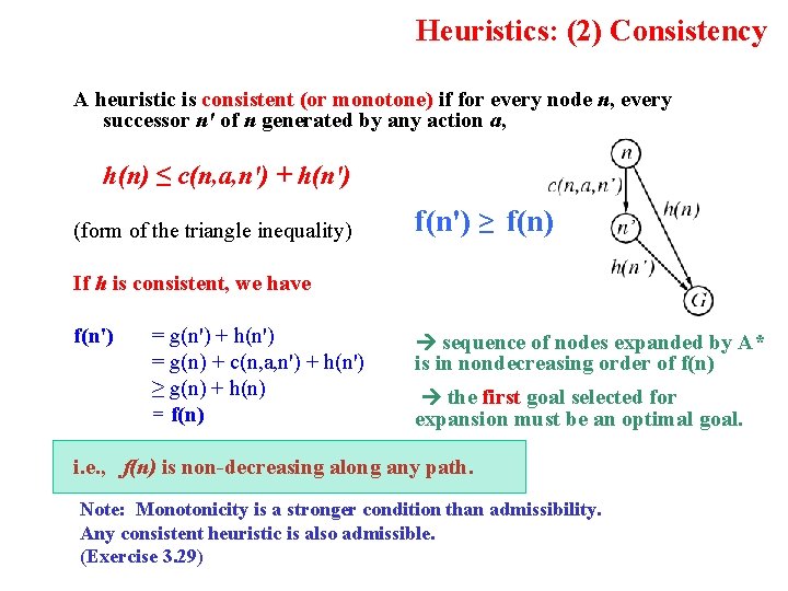
Heuristics: (2) Consistency A heuristic is consistent (or monotone) if for every node n, every successor n' of n generated by any action a, h(n) ≤ c(n, a, n') + h(n') (form of the triangle inequality) f(n') ≥ f(n) If h is consistent, we have f(n') = g(n') + h(n') = g(n) + c(n, a, n') + h(n') ≥ g(n) + h(n) = f(n) sequence of nodes expanded by A* is in nondecreasing order of f(n) the first goal selected for expansion must be an optimal goal. i. e. , f(n) is non-decreasing along any path. Note: Monotonicity is a stronger condition than admissibility. Any consistent heuristic is also admissible. (Exercise 3. 29)
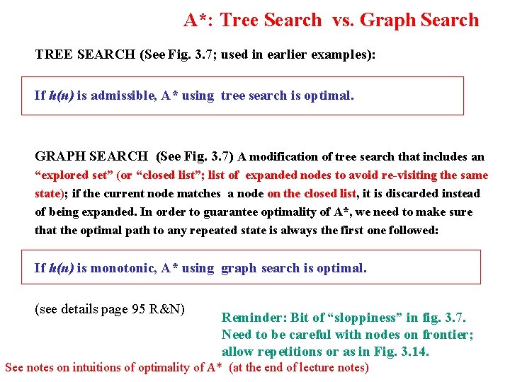
A*: Tree Search vs. Graph Search TREE SEARCH (See Fig. 3. 7; used in earlier examples): If h(n) is admissible, A* using tree search is optimal. GRAPH SEARCH (See Fig. 3. 7) A modification of tree search that includes an “explored set” (or “closed list”; list of expanded nodes to avoid re-visiting the same state); if the current node matches a node on the closed list, it is discarded instead of being expanded. In order to guarantee optimality of A*, we need to make sure that the optimal path to any repeated state is always the first one followed: If h(n) is monotonic, A* using graph search is optimal. (see details page 95 R&N) Reminder: Bit of “sloppiness” in fig. 3. 7. Need to be careful with nodes on frontier; allow repetitions or as in Fig. 3. 14. See notes on intuitions of optimality of A* (at the end of lecture notes)
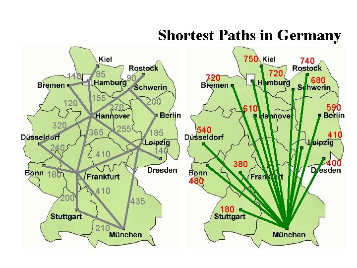
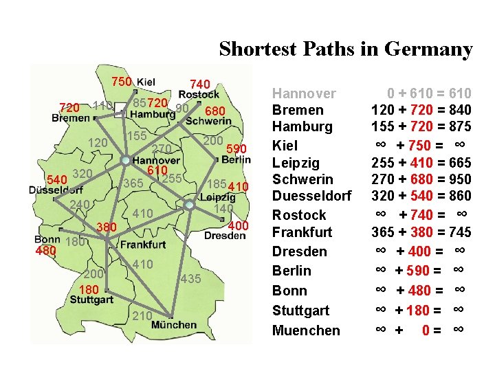
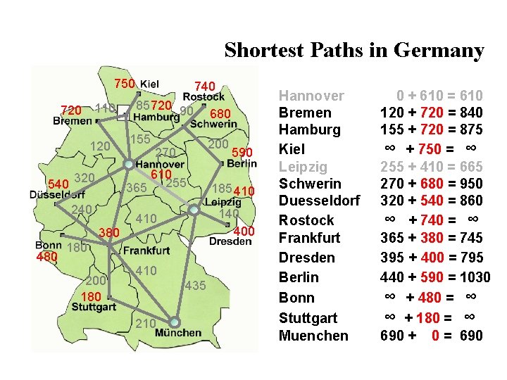
Example: Contrasting A* with Uniform Cost (Dijkstra’s algorithm) Example: The shortest route from Hannover to Munich 1) Dijkstra’s alg. , i. e. , A* with h(n)=0 (Uniform cost search) 2) A* search Example thanks to Meinolf Sellmann
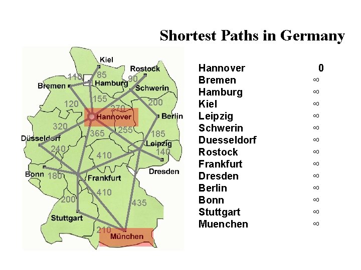
Shortest Paths in Germany 110 120 320 240 85 155 90 200 270 365 255 140 410 180 200 410 435 210 185 Hannover Bremen Hamburg Kiel Leipzig Schwerin Duesseldorf Rostock Frankfurt Dresden Berlin Bonn Stuttgart Muenchen 0 ∞ ∞ ∞ ∞
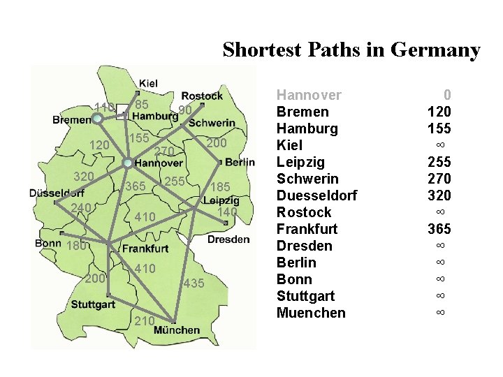
Shortest Paths in Germany 110 120 320 240 85 155 90 200 270 365 255 140 410 180 200 410 435 210 185 Hannover Bremen Hamburg Kiel Leipzig Schwerin Duesseldorf Rostock Frankfurt Dresden Berlin Bonn Stuttgart Muenchen 0 120 155 ∞ 255 270 320 ∞ 365 ∞ ∞ ∞
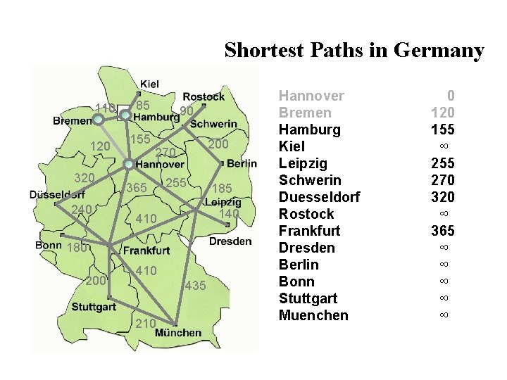
Shortest Paths in Germany 110 120 320 240 85 155 90 200 270 365 255 140 410 180 200 410 435 210 185 Hannover Bremen Hamburg Kiel Leipzig Schwerin Duesseldorf Rostock Frankfurt Dresden Berlin Bonn Stuttgart Muenchen 0 120 155 ∞ 255 270 320 ∞ 365 ∞ ∞ ∞
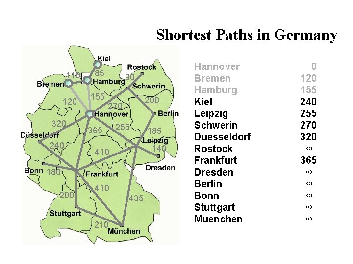
Shortest Paths in Germany 110 120 320 240 85 155 90 200 270 365 255 140 410 180 200 410 435 210 185 Hannover Bremen Hamburg Kiel Leipzig Schwerin Duesseldorf Rostock Frankfurt Dresden Berlin Bonn Stuttgart Muenchen 0 120 155 240 255 270 320 ∞ 365 ∞ ∞ ∞

Shortest Paths in Germany 110 120 320 240 85 155 90 200 270 365 255 140 410 180 200 410 435 210 185 Hannover Bremen Hamburg Kiel Leipzig Schwerin Duesseldorf Rostock Frankfurt Dresden Berlin Bonn Stuttgart Muenchen 0 120 155 240 255 270 320 ∞ 365 ∞ ∞ ∞
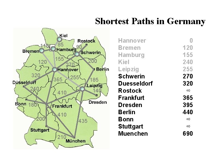
Shortest Paths in Germany 110 120 320 240 85 155 90 200 270 365 255 140 410 180 200 410 435 210 185 Hannover Bremen Hamburg Kiel Leipzig Schwerin Duesseldorf Rostock Frankfurt Dresden Berlin Bonn Stuttgart Muenchen 0 120 155 240 255 270 320 ∞ 365 395 440 ∞ ∞ 690
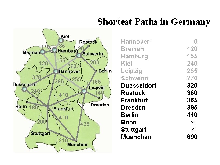
Shortest Paths in Germany 110 120 320 240 85 155 90 200 270 365 255 140 410 180 200 410 435 210 185 Hannover Bremen Hamburg Kiel Leipzig Schwerin Duesseldorf Rostock Frankfurt Dresden Berlin Bonn Stuttgart Muenchen 0 120 155 240 255 270 320 365 395 440 ∞ ∞ 690
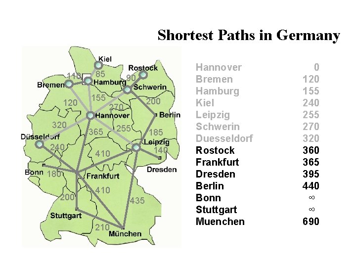
Shortest Paths in Germany 110 120 320 240 85 155 90 200 270 365 255 140 410 180 200 410 435 210 185 Hannover Bremen Hamburg Kiel Leipzig Schwerin Duesseldorf Rostock Frankfurt Dresden Berlin Bonn Stuttgart Muenchen 0 120 155 240 255 270 320 365 395 440 ∞ ∞ 690
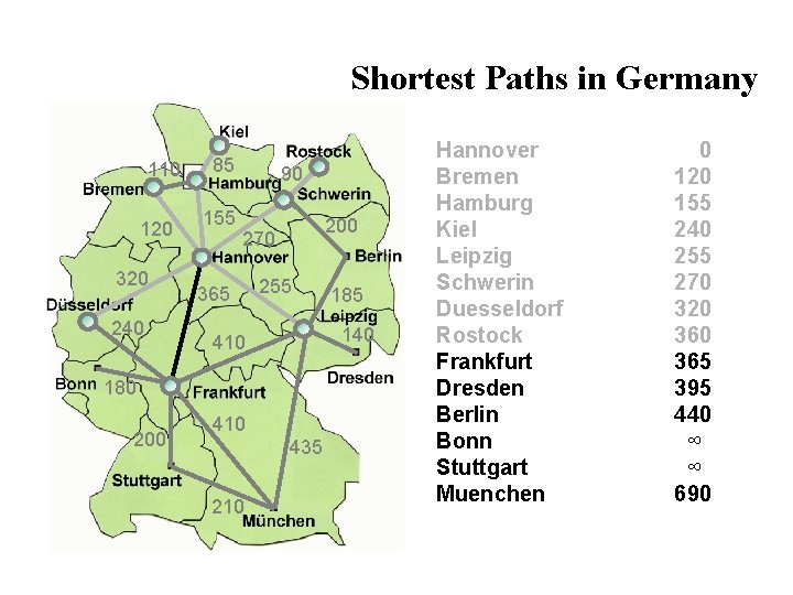
Shortest Paths in Germany 110 120 320 240 85 155 90 200 270 365 255 140 410 180 200 410 435 210 185 Hannover Bremen Hamburg Kiel Leipzig Schwerin Duesseldorf Rostock Frankfurt Dresden Berlin Bonn Stuttgart Muenchen 0 120 155 240 255 270 320 365 395 440 ∞ ∞ 690
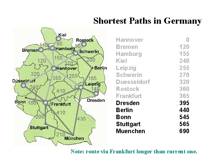
Shortest Paths in Germany 110 120 320 240 85 155 90 200 270 365 255 140 410 180 200 410 435 210 185 Hannover Bremen Hamburg Kiel Leipzig Schwerin Duesseldorf Rostock Frankfurt Dresden Berlin Bonn Stuttgart Muenchen 0 120 155 240 255 270 320 365 395 440 545 565 690 Note: route via Frankfurt longer than current one.

Shortest Paths in Germany 110 120 320 240 85 155 90 200 270 365 255 140 410 180 200 410 435 210 185 Hannover Bremen Hamburg Kiel Leipzig Schwerin Duesseldorf Rostock Frankfurt Dresden Berlin Bonn Stuttgart Muenchen 0 120 155 240 255 270 320 365 395 440 545 565 690
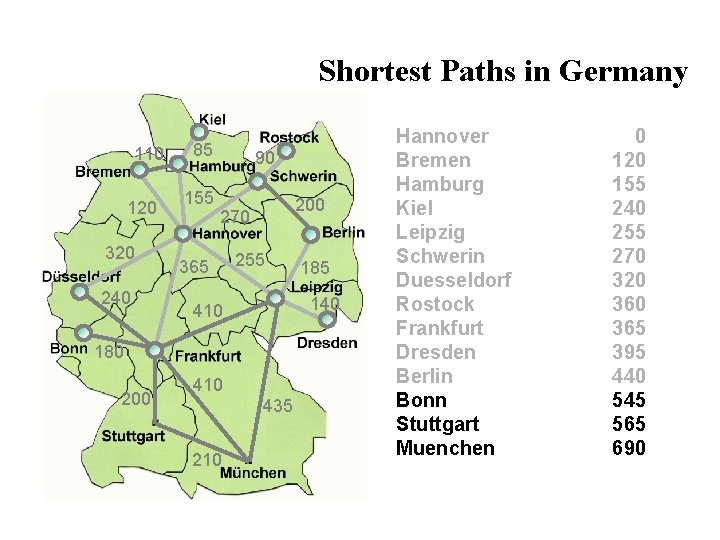
Shortest Paths in Germany 110 120 320 240 85 155 90 200 270 365 255 140 410 180 200 410 435 210 185 Hannover Bremen Hamburg Kiel Leipzig Schwerin Duesseldorf Rostock Frankfurt Dresden Berlin Bonn Stuttgart Muenchen 0 120 155 240 255 270 320 365 395 440 545 565 690
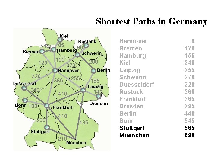
Shortest Paths in Germany 110 120 320 240 85 155 90 200 270 365 255 140 410 180 200 410 435 210 185 Hannover Bremen Hamburg Kiel Leipzig Schwerin Duesseldorf Rostock Frankfurt Dresden Berlin Bonn Stuttgart Muenchen 0 120 155 240 255 270 320 365 395 440 545 565 690
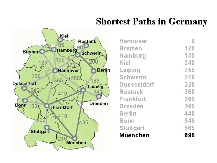
Shortest Paths in Germany 110 120 320 240 85 155 90 200 270 365 255 140 410 180 200 410 435 210 185 Hannover Bremen Hamburg Kiel Leipzig Schwerin Duesseldorf Rostock Frankfurt Dresden Berlin Bonn Stuttgart Muenchen 0 120 155 240 255 270 320 365 395 440 545 565 690
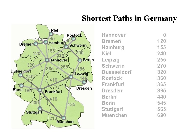
Shortest Paths in Germany 110 120 320 240 85 155 90 200 270 365 255 140 410 180 200 410 435 210 185 Hannover Bremen Hamburg Kiel Leipzig Schwerin Duesseldorf Rostock Frankfurt Dresden Berlin Bonn Stuttgart Muenchen 0 120 155 240 255 270 320 365 395 440 545 565 690
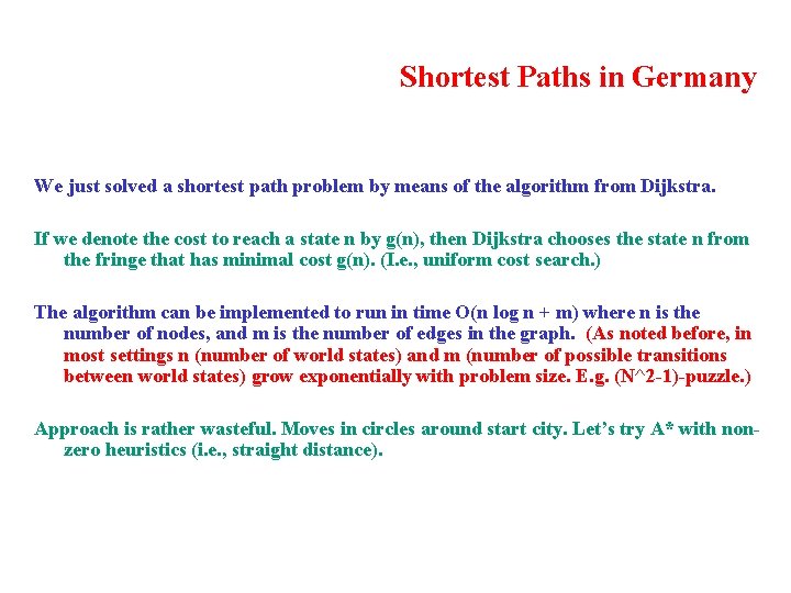
Shortest Paths in Germany We just solved a shortest path problem by means of the algorithm from Dijkstra. If we denote the cost to reach a state n by g(n), then Dijkstra chooses the state n from the fringe that has minimal cost g(n). (I. e. , uniform cost search. ) The algorithm can be implemented to run in time O(n log n + m) where n is the number of nodes, and m is the number of edges in the graph. (As noted before, in most settings n (number of world states) and m (number of possible transitions between world states) grow exponentially with problem size. E. g. (N^2 -1)-puzzle. ) Approach is rather wasteful. Moves in circles around start city. Let’s try A* with nonzero heuristics (i. e. , straight distance).
Shortest Paths in Germany 750 110 120 320 240 85 155 200 270 365 255 185 610 540 590 410 380 410 435 210 680 140 410 180 200 720 90 740 180 400
Shortest Paths in Germany 750 110 720 120 540 85 720 90 155 380 410 435 210 590 185 410 140 400 410 180 200 180 680 200 270 610 365 255 320 240 480 740 Hannover Bremen Hamburg Kiel Leipzig Schwerin Duesseldorf Rostock Frankfurt Dresden Berlin Bonn Stuttgart Muenchen 0 + 610 = 610 120 + 720 = 840 155 + 720 = 875 ∞ + 750 = ∞ 255 + 410 = 665 270 + 680 = 950 320 + 540 = 860 ∞ + 740 = ∞ 365 + 380 = 745 ∞ + 400 = ∞ ∞ + 590 = ∞ ∞ + 480 = ∞ ∞ + 180 = ∞ ∞ + 0= ∞
Shortest Paths in Germany 750 110 720 120 540 85 720 90 155 380 410 435 210 590 185 410 140 400 410 180 200 180 680 200 270 610 365 255 320 240 480 740 Hannover Bremen Hamburg Kiel Leipzig Schwerin Duesseldorf Rostock Frankfurt Dresden Berlin Bonn Stuttgart Muenchen 0 + 610 = 610 120 + 720 = 840 155 + 720 = 875 ∞ + 750 = ∞ 255 + 410 = 665 270 + 680 = 950 320 + 540 = 860 ∞ + 740 = ∞ 365 + 380 = 745 395 + 400 = 795 440 + 590 = 1030 ∞ + 480 = ∞ ∞ + 180 = ∞ 690 + 0 = 690
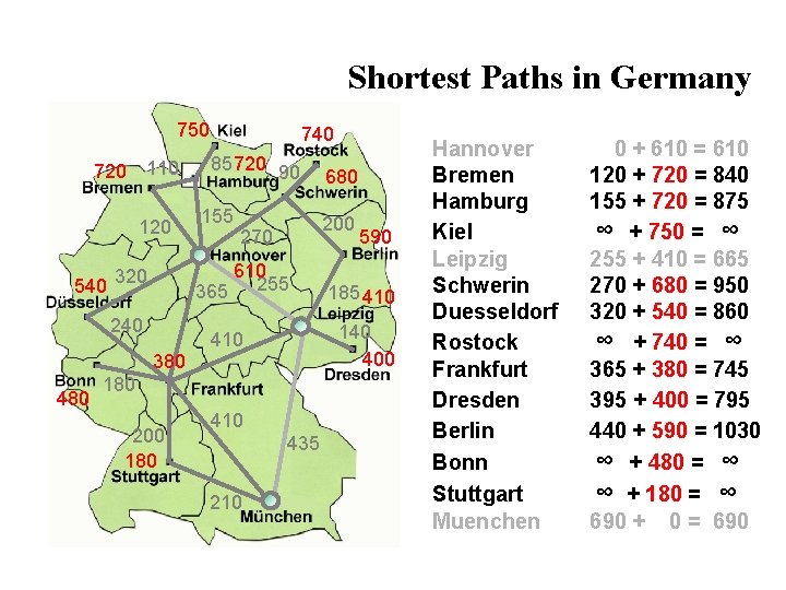
Shortest Paths in Germany 750 110 720 120 540 85 720 90 155 380 410 435 210 590 185 410 140 400 410 180 200 180 680 200 270 610 365 255 320 240 480 740 Hannover Bremen Hamburg Kiel Leipzig Schwerin Duesseldorf Rostock Frankfurt Dresden Berlin Bonn Stuttgart Muenchen 0 + 610 = 610 120 + 720 = 840 155 + 720 = 875 ∞ + 750 = ∞ 255 + 410 = 665 270 + 680 = 950 320 + 540 = 860 ∞ + 740 = ∞ 365 + 380 = 745 395 + 400 = 795 440 + 590 = 1030 ∞ + 480 = ∞ ∞ + 180 = ∞ 690 + 0 = 690
Heuristics
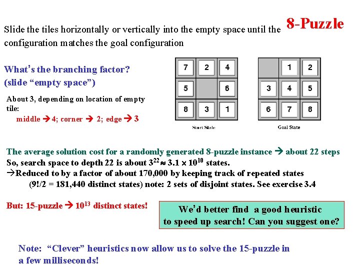
Slide the tiles horizontally or vertically into the empty space until the configuration matches the goal configuration 8 -Puzzle What’s the branching factor? (slide “empty space”) About 3, depending on location of empty tile: middle 4; corner 2; edge 3 The average solution cost for a randomly generated 8 -puzzle instance about 22 steps So, search space to depth 22 is about 322 3. 1 1010 states. Reduced to by a factor of about 170, 000 by keeping track of repeated states (9!/2 = 181, 440 distinct states) note: 2 sets of disjoint states. See exercise 3. 4 But: 15 -puzzle 1013 distinct states! We’d better find a good heuristic to speed up search! Can you suggest one? Note: “Clever” heuristics now allow us to solve the 15 -puzzle in a few milliseconds!
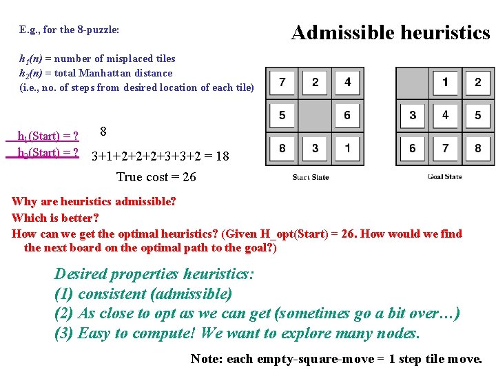
Admissible heuristics E. g. , for the 8 -puzzle: h 1(n) = number of misplaced tiles h 2(n) = total Manhattan distance (i. e. , no. of steps from desired location of each tile) h 1(Start) = ? h 2(Start) = ? 8 3+1+2+2+2+3+3+2 = 18 True cost = 26 Why are heuristics admissible? Which is better? How can we get the optimal heuristics? (Given H_opt(Start) = 26. How would we find the next board on the optimal path to the goal? ) Desired properties heuristics: (1) consistent (admissible) (2) As close to opt as we can get (sometimes go a bit over…) (3) Easy to compute! We want to explore many nodes. Note: each empty-square-move = 1 step tile move.
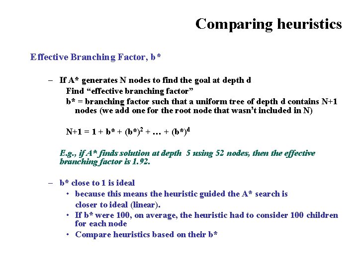
Comparing heuristics Effective Branching Factor, b* – If A* generates N nodes to find the goal at depth d Find “effective branching factor” b* = branching factor such that a uniform tree of depth d contains N+1 nodes (we add one for the root node that wasn’t included in N) N+1 = 1 + b* + (b*)2 + … + (b*)d E. g. , if A* finds solution at depth 5 using 52 nodes, then the effective branching factor is 1. 92. – b* close to 1 is ideal • because this means the heuristic guided the A* search is closer to ideal (linear). • If b* were 100, on average, the heuristic had to consider 100 children for each node • Compare heuristics based on their b*
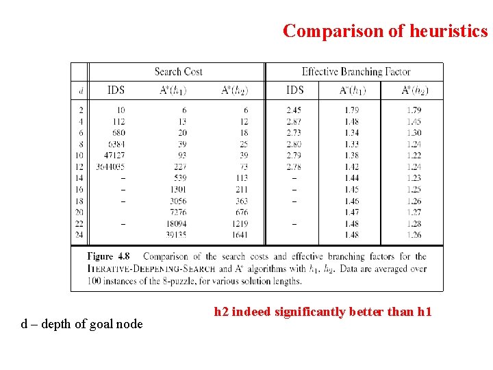
Comparison of heuristics d – depth of goal node h 2 indeed significantly better than h 1
Dominating heuristics h 2 is always better than h 1 – Because for any node, n, h 2(n) >= h 1(n). (Why? ) We say h 2 dominates h 1 It follows that h 1 will expand at least as many nodes as h 2. Because: Recall nodes with f(n) < C* will be expanded. This means all nodes, h(n) + g(n) < C*, will be expanded. So, all nodes n where h(n) < C* - g(n) will be expanded All nodes h 2 expands will also be expanded by h 1 and because h 1 is smaller, others may be expanded as well
Inventing admissible heuristics: Relaxed Problems Can we generate h(n) automatically? – Simplify problem by reducing restrictions on actions A problem with fewer restrictions on the actions is called a relaxed problem
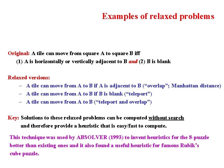
Examples of relaxed problems Original: A tile can move from square A to square B iff (1) A is horizontally or vertically adjacent to B and (2) B is blank Relaxed versions: – A tile can move from A to B if A is adjacent to B (“overlap”; Manhattan distance) – A tile can move from A to B if B is blank (“teleport”) – A tile can move from A to B (“teleport and overlap”) Key: Solutions to these relaxed problems can be computed without search and therefore provide a heuristic that is easy/fast to compute. This technique was used by ABSOLVER (1993) to invent heuristics for the 8 -puzzle better than existing ones and it also found a useful heuristic for famous Rubik’s cube puzzle.
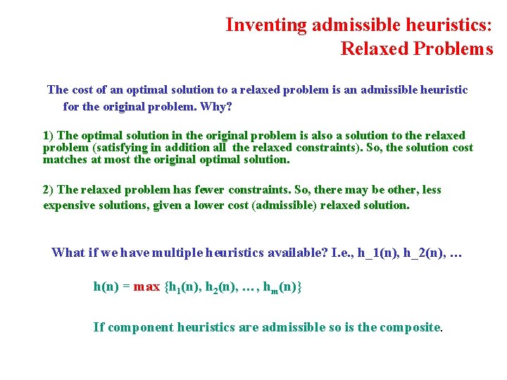
Inventing admissible heuristics: Relaxed Problems The cost of an optimal solution to a relaxed problem is an admissible heuristic for the original problem. Why? 1) The optimal solution in the original problem is also a solution to the relaxed problem (satisfying in addition all the relaxed constraints). So, the solution cost matches at most the original optimal solution. 2) The relaxed problem has fewer constraints. So, there may be other, less expensive solutions, given a lower cost (admissible) relaxed solution. What if we have multiple heuristics available? I. e. , h_1(n), h_2(n), … h(n) = max {h 1(n), h 2(n), …, hm(n)} If component heuristics are admissible so is the composite.

Inventing admissible heuristics: Learning Also automatically learning admissible heuristics using machine learning techniques, e. g. , inductive learning and reinforcement learning. Generally, you try to learn a “state-evaluation” function or “board evaluation” function. (How desirable is state in terms of getting to the goal? ) Key: What “features / properties” of state are most useful? More later…
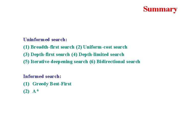
Summary Uninformed search: (1) Breadth-first search (2) Uniform-cost search (3) Depth-first search (4) Depth-limited search (5) Iterative deepening search (6) Bidirectional search Informed search: (1) Greedy Best-First (2) A*
Summary, cont. Heuristics allow us to scale up solutions dramatically! Can now search combinatorial (exponential size) spaces with easily 10^15 states and even up to 10^100 or more states. Especially, in modern heuristics search planners (eg FF). Before informed search, considered totally infeasible. Still many variations and subtleties: There are conferences and journals dedicated solely to search. Lots of variants of A*. Research in A* has increased dramatically since A* is the key algorithm used by map engines. Also used in path planning algorithms (autonomous vehicles), and general (robotics) planning, problem solving, and even NLP parsing. The end
A*: Tree Search vs. Graph Search TREE SEARCH (See Fig. 3. 7; used in earlier examples): If h(n) is admissible, A* using tree search is optimal. GRAPH SEARCH (See Fig. 3. 7) A modification of tree search that includes an “explored set” (or “closed list”; list of expanded nodes to avoid re-visiting the same state); if the current node matches a node on the closed list, it is discarded instead of being expanded. In order to guarantee optimality of A*, we need to make sure that the optimal path to any repeated state is always the first one followed: If h(n) is monotonic, A* using graph search is optimal. (proof next) (see details page 95 R&N) Reminder: Bit of “sloppiness” in fig. 3. 7. Need to be careful with nodes on frontier; allow repetitions or as in Fig. 3. 14.
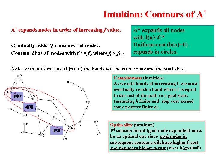
Intuition: Contours of A* A* expands nodes in order of increasing f value. Gradually adds "f-contours" of nodes. Contour i has all nodes with f <= fi, where fi < fi+1 A* expands all nodes with f(n)<C* Uniform-cost (h(n)=0) expands in circles. Note: with uniform cost (h(n)=0) the bands will be circular around the start state. Completeness (intuition) As we add bands of increasing f, we must eventually reach a band where f is equal to the cost of the path to a goal state. (assuming b finite and step cost exceed some positive finite ε). 380 400 420 Optimality (intuition) 1 st solution found (goal node expanded) must be an optimal one since goal nodes in subsequent contours will have higher f-cost and therefore higher g-cost (since h(goal)=0)
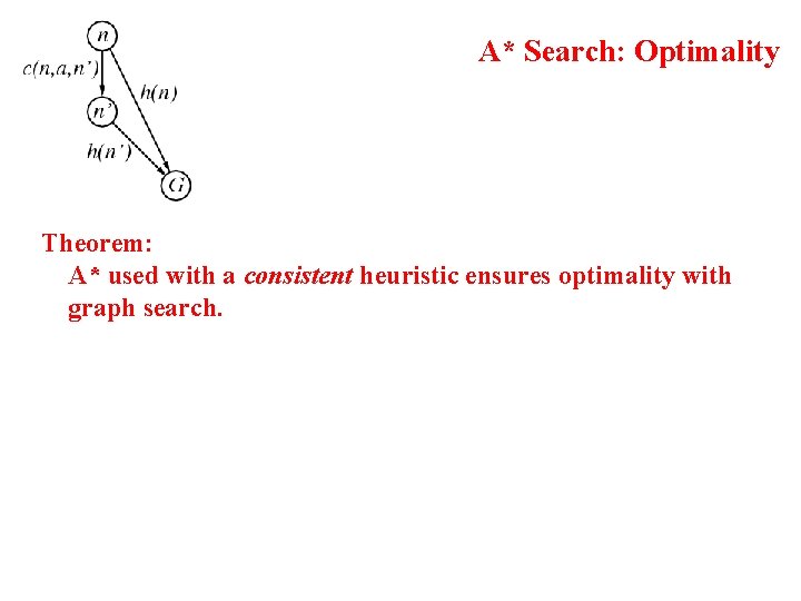
A* Search: Optimality Theorem: A* used with a consistent heuristic ensures optimality with graph search.
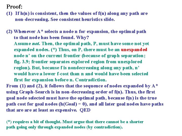
Proof: (1) If h(n) is consistent, then the values of f(n) along any path are non-decreasing. See consistent heuristics slide. (2) Whenever A* selects a node n for expansion, the optimal path to that node has been found. Why? Assume not. Then, the optimal path, P, must have some not yet expanded nodes. (*) Thus, on P, there must be an unexpanded node n’ on the current frontier (because of graph separation; fig. 3. 9; frontier separates explored region from unexplored region). But, because f is nondecreasing along any path, n’ would have a lower f-cost than n and would have been selected first for expansion before n. Contradiction. From (1) and (2), it follows that the sequence of nodes expanded by A* using Graph-Search is in non-decreasing order of f(n). Thus, the first goal node selected must have the optimal path, because f(n) is the true path cost for goal nodes (h(Goal) = 0), and all later goal nodes have paths that are at least as expensive. QED (*) requires a bit of thought. Must argue that there cannot be a shorter path going only through expanded nodes (by contradiction).
Note: Termination / Completeness Termination is guaranteed when the number of nodes with is finite. Non-termination can only happen when – There is a node with an infinite branching factor, or – There is a path with a finite cost but an infinite number of nodes along it. • Can be avoided by assuming that the cost of each action is larger than a positive constant d
A* Optimal in Another Way It has also been shown that A* makes optimal use of the heuristics in the sense that there is no search algorithm that could expand fewer nodes using the heuristic information (and still find the optimal / least cost solution. So, A* is “the best we can get. ” Note: We’re assuming a search based approach with states/nodes, actions on them leading to other states/nodes, start and goal states/nodes.
- Slides: 62