Correlation and Regression History 5011 Sir Francis Galton

Correlation and Regression History 5011

Sir Francis Galton 1822 -1911 Geographer, meteorologist, tropical explorer, inventor of fingerprint identification, eugenicist, half-cousin of Charles Darwin and best-selling author.

Galton n Obsessed with measurement Tried to measure everything from the weather to female beauty Invented correlation and regression

Sweet Peas Galton’s experiment with sweet peas (1875) led to the development of initial concepts of linear regression. n Sweet peas could self-fertilize: “daughter plants express genetic variations from mother plants without contribution from a second parent. ” n

Sweet Peas (2) n n n Distributed packets of seeds to 7 friends Uniformly distributed sizes, split into 7 size groups with 10 seeds per size. There was substantial variation among packets. 7 sizes 10 seeds per size 7 friends = 490 seeds Friends were to harvest seeds from the new generation of friends and return them to Galton.

Sweet Peas (3) Plotted the weights of daughter seeds against weights of mother seeds. n Hand fitted a line to the data n Slope of the line connecting the means of different columns is equivalent to regression slope. n

Sweet Pea Scatterplot

Sweet Pea Scatterplot with Regression Line

Slope indicates strength of association Galton drew his line by hand, and estimated that for every thousandth of an inch of increased size of parents, the daughters size was affected by. 33 thousandths.

Things Galton Noticed n n Mother plants of a given seed size tended to have daughter seeds of pretty similar sizes Extremely large mother seeds grew into plants whose daughter seeds were generally not so large Extremely small mother seeds grew into plants whose daughter seeds were generally not so small Galton put a name on the loss of extremity: “Regression to the mean”

Karl Pearson (1857 -1936) n n Formalized Galton’s method Invented least squares method of determining regression line Pearson with Galton, c. 1900

Least squares idea: Choose the line that minimizes the sum of the squares of the deviations of each observation from the regression line

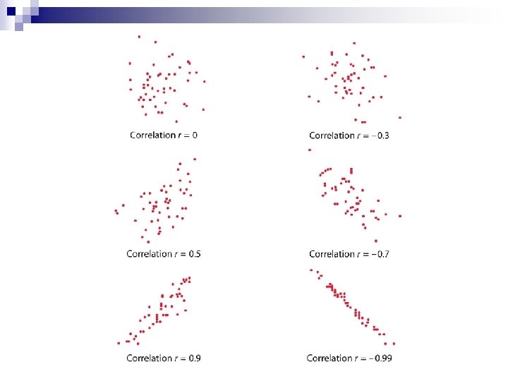
Scatterplots Example 1 Example 2 Example 3 Example 4 Example 5

Correlations: Positive Large values of X associated with large values of Y, small values of X associated with small values of Y. e. g. IQ and SAT Negative Large values of X associated with small values of Y & vice versa e. g. SPEED and ACCURACY

Correlation does not imply causality § § § Two variables might be associated because they share a common cause. For example, SAT scores and College Grade are highly associated, but probably not because scoring well on the SAT causes a student to get high grades in college. Being a good student, etc. , would be the common cause of the SATs and the grades.

Intervening and confounding factors There is a positive correlation between ice cream sales and drownings. There is a strong positive association between Number of Years of Education and Annual Income § In part, getting more education allows people to get better, higher-paying jobs. § But these variables are confounded with others, such as socio-economic status

Regression and correlation will not capture nonlinear relationships

Speed And Mileage Have A Curved Relationship. Using r would be inappropriate MILEAGE* FUEL CONSUMPTION & SPEED r = -0. 172 SPEED (KM/H) * Mileage: liters / 100 km

Bivariate regression equation Y=bx+c b=slope c=intercept

Adding another variable

Multiple regression equation Y=b 1 x 1+b 2 x 2+ c b 1=slope of 1 st variable X 1=1 st variable B 2=slope of 2 nd variable X 2=second variable c=intercept

Another view

Another view

Dummy variables n n All examples have been continuous variables, but most historical data is categorical We can recode categorical variables into dummy variables Race becomes codes white (0, 1) black (0, 1) Asian (0, 1) One category must be omitted

Dummy variable scatter plot (FEV is forced expiratory volume)

Bivariate regression results ß Variable (coefficient F-test SMOKE 0. 71 41. 7892 Y-Intercept 2. 5661426 n The slope coefficient of 0. 71 for SMOKE and FEV suggests hat FEV increases 0. 71 units (on the average) as we go from SMOKE = 0 (nonsmoker) to SMOKE = 1 (smoker). This is surprisingly given what we know about smoking. How can a positive relation between SMOKE and FEV exist given what we know about the physiological effects of smoking? The answer lies in understanding the confounding effects of AGE on SMOKE and FEV. In this child and adolescent population, nonsmokers are younger than nonsmokers (mean ages: 9. 5 years vs. 13. 5 years, respectively). It is therefore not surprising that AGE confounds the relation between SMOKE and FEV. So what are we to do?

Dummy variable scatterplot (3 -D)

Multiple regression results

Intergenerational coresidence of the aged, 1950 -2000: Independent variables

State-level regression results