Chapter 4 The Heckscher Ohlin Model Topics to

Chapter 4 The Heckscher. Ohlin Model

Topics to be Covered • The Heckscher-Ohlin (HO) Model: Basic Assumptions • The HO Theorem • Equilibrium in the HO model • Some New HO Theorems • Some Final Observations © 2013 Pearson Education, Inc. All rights reserved. 4 -2

Heckscher-Ohlin (HO) Model • Developed by Eli Heckscher and Bertil Ohlin, Swedish economists. • Model based on two concepts: 1. Factor endowments—the quantities of productive resources possessed by a country 2. Factor intensity—the amount of labor per unit of capital used in production of a product © 2013 Pearson Education, Inc. All rights reserved. 4 -3

Assumptions of HO Model • Keep first 10 assumptions (from chapters 2 and 3) • Drop assumptions 11 (labor is only resource) and 12 (constant returns to scale) • Add five new assumptions © 2013 Pearson Education, Inc. All rights reserved. 4 -4

Five New Assumptions • Assumption 13—Two resources, labor (L) and capital (K), and resource payments, wages for labor (W) and rent for capital (R) • Assumption 14—Identical technology in both countries; choice of production technique depends on factor prices (Note: this assumption rules out the classical basis for international trade) © 2013 Pearson Education, Inc. All rights reserved. 4 -5

Assumption 15 • Assumption 15—Production of good T is more labor-intensive than that of good S. Production of both goods in both countries is subject to constant returns to scale. © 2013 Pearson Education, Inc. All rights reserved. 4 -6

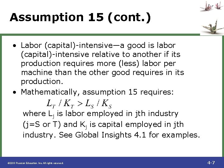
Assumption 15 (cont. ) • Labor (capital)-intensive—a good is labor (capital)-intensive relative to another if its production requires more (less) labor per machine than the other good requires in its production. • Mathematically, assumption 15 requires: where Lj is labor employed in jth industry (j=S or T) and Kj is capital employed in jth industry. See Global Insights 4. 1 for examples. © 2013 Pearson Education, Inc. All rights reserved. 4 -7

Assumption 16 • Assumption 16—Country A is relatively capital-abundant while B is relatively laborabundant. • Two definitions of resource abundance: – Quantity definition – Price definition © 2013 Pearson Education, Inc. All rights reserved. 4 -8

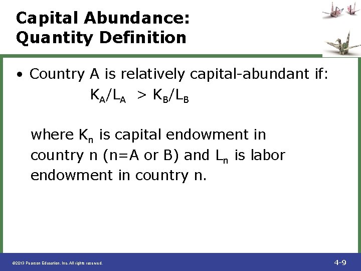
Capital Abundance: Quantity Definition • Country A is relatively capital-abundant if: KA/LA > KB/LB where Kn is capital endowment in country n (n=A or B) and Ln is labor endowment in country n. © 2013 Pearson Education, Inc. All rights reserved. 4 -9

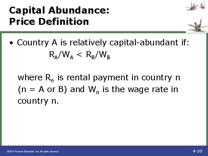
Capital Abundance: Price Definition • Country A is relatively capital-abundant if: RA/WA < RB/WB where Rn is rental payment in country n (n = A or B) and Wn is the wage rate in country n. © 2013 Pearson Education, Inc. All rights reserved. 4 -10

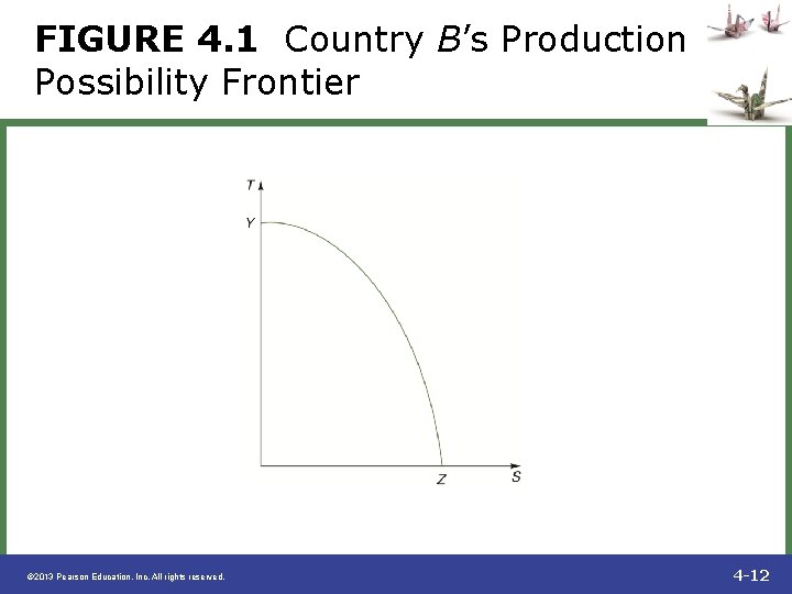
Production Possibility Frontier • Since the two goods differ in factor intensity in both countries, the PPFs of each country will exhibit increasing opportunity cost (i. e. , PPF will have a bowed out, nonlinear shape). • Because country B is labor-abundant and good T is labor-intensive, B’s PPF will lie primarily along (or biased toward) the Taxis (see Figure 4. 1). © 2013 Pearson Education, Inc. All rights reserved. 4 -11

FIGURE 4. 1 Country B’s Production Possibility Frontier © 2013 Pearson Education, Inc. All rights reserved. 4 -12

Assumption 17 • Tastes in the two countries are identical. That is, both countries have the same set of community indifference curves (CIC). • This assumption guarantees that a country’s comparative advantage is determined primarily by supply, not demand, factors. © 2013 Pearson Education, Inc. All rights reserved. 4 -13

Heckscher-Ohlin Theorem • A country will have comparative advantage in, and therefore will export, that good whose production is relatively intensive in the factor with which the country is relatively well-endowed. © 2013 Pearson Education, Inc. All rights reserved. 4 -14

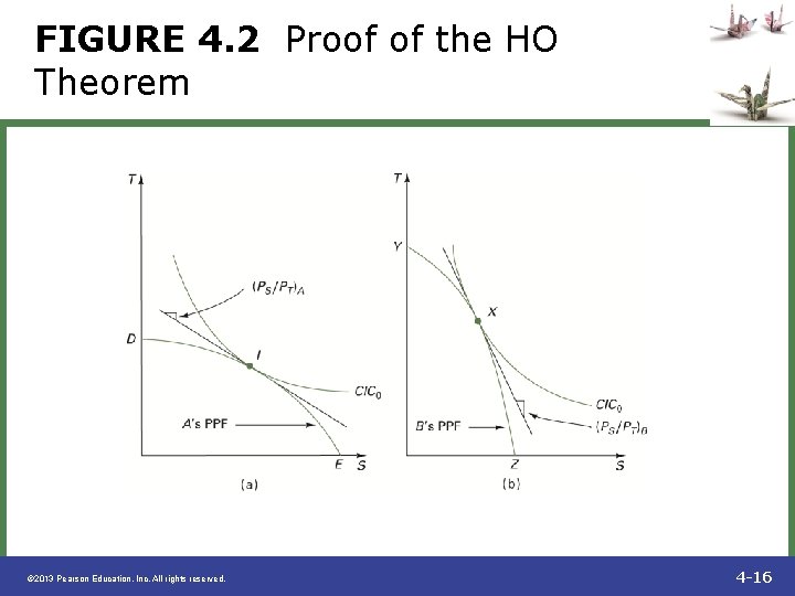
Graphical Proof of HO Theorem • Given different PPFs for the two countries and identical CICs, find autarky equilibrium points for both countries (see Figure 4. 2) • At the equilibrium point, the slope of each country’s PPF equals the pre-trade price ratio • Since (PS /PT )A < (PS /PT )B , then A(B) has comparative advantage in, and will export, good S(T) © 2013 Pearson Education, Inc. All rights reserved. 4 -15

FIGURE 4. 2 Proof of the HO Theorem © 2013 Pearson Education, Inc. All rights reserved. 4 -16

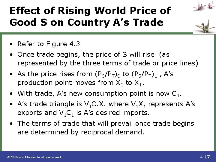
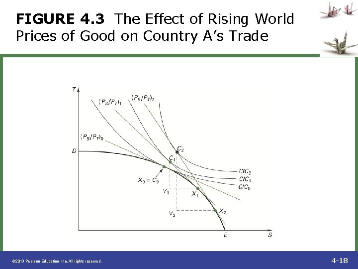
Effect of Rising World Price of Good S on Country A’s Trade • Refer to Figure 4. 3 • Once trade begins, the price of S will rise (as represented by the three terms of trade or price lines) • As the price rises from (PS/PT)0 to (PS/PT)1 , A’s production point moves from X 0 to X 1. • With trade, A’s new consumption point is now C 1. • A’s trade triangle is V 1 C 1 X 1 where V 1 X 1 represents A’s exports and V 1 C 1 is A’s desired imports. • The terms of trade that will prevail once trade begins are determined by reciprocal demand. © 2013 Pearson Education, Inc. All rights reserved. 4 -17

FIGURE 4. 3 The Effect of Rising World Prices of Good on Country A’s Trade © 2013 Pearson Education, Inc. All rights reserved. 4 -18

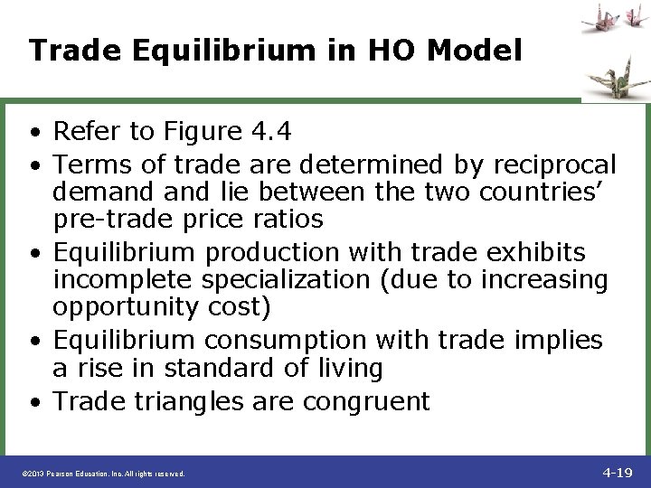
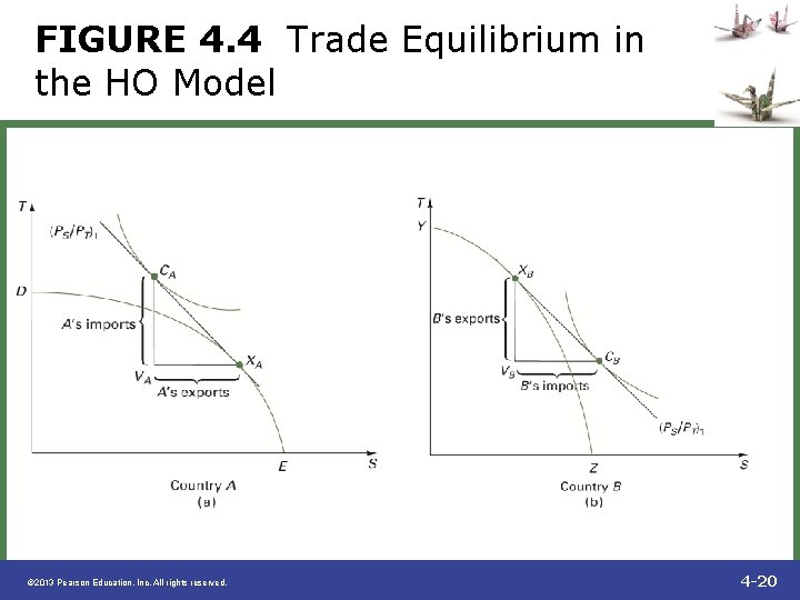
Trade Equilibrium in HO Model • Refer to Figure 4. 4 • Terms of trade are determined by reciprocal demand lie between the two countries’ pre-trade price ratios • Equilibrium production with trade exhibits incomplete specialization (due to increasing opportunity cost) • Equilibrium consumption with trade implies a rise in standard of living • Trade triangles are congruent © 2013 Pearson Education, Inc. All rights reserved. 4 -19

FIGURE 4. 4 Trade Equilibrium in the HO Model © 2013 Pearson Education, Inc. All rights reserved. 4 -20

Differences between Classical and HO Models • Complete specialization results in classical model, while incomplete specialization occurs in HO model. • In classical model, only demand conditions affect reciprocal demand. In HO model, reciprocal demand leads to equilibrium price via changes in both demand supply. • Autarky price in the classical model is determined only by supply conditions. In HO model, demand supply determine autarky price. © 2013 Pearson Education, Inc. All rights reserved. 4 -21

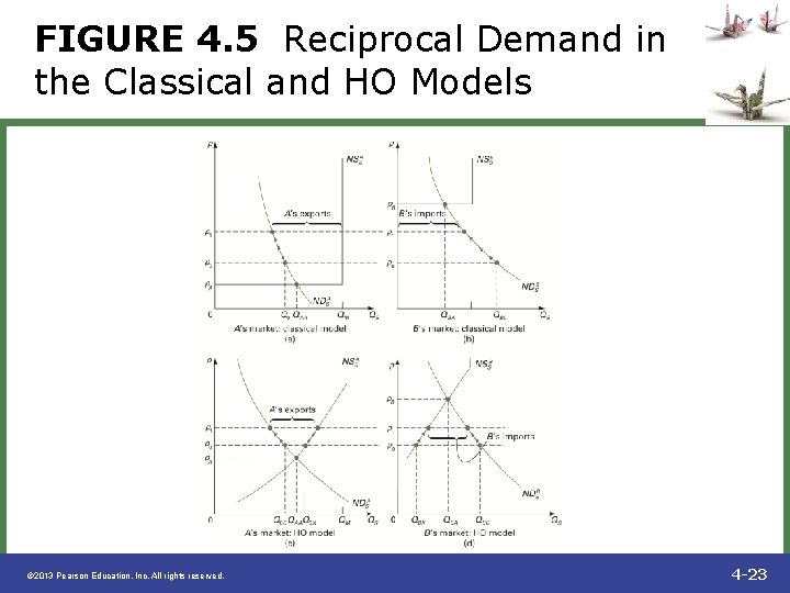
Reciprocal Demand in the Classical and HO Models • Refer to Figure 4. 5 • The national supply curves differ in the two models. In the classical model, the national supply curve is horizontal (due to constant cost) up to the point of complete specialization, at which the curve becomes vertical. In the HO model, the curve is initially upward-sloping (due to increasing costs). • Autarky equilibrium is achieved where the national demand national supply curves intersect. Since the relative price PS/PT is lower in country A, then A has a comparative advantage in good S. © 2013 Pearson Education, Inc. All rights reserved. 4 -22

FIGURE 4. 5 Reciprocal Demand in the Classical and HO Models © 2013 Pearson Education, Inc. All rights reserved. 4 -23

Reciprocal Demand (Classical Model) • See Figures 4. 5 a and 4. 5 b. • When trade begins at a world price p 0, A’s production of S rises to its complete specialization level and A exports what it does not consume. In country B, production of S falls to zero and its imports of S increase. • Due to excess demand at p 0, the world price will rise and consumption in both countries will fall until the world markets attain equilibrium at new world price p 1. © 2013 Pearson Education, Inc. All rights reserved. 4 -24

Reciprocal Demand (HO Model) • See Figures 4. 5 c and 4. 5 d • Similar to the Classical model except in how the excess demand is eliminated. As the world price rises in response to the excess demand, consumption falls in both countries but supply also rises in both countries. © 2013 Pearson Education, Inc. All rights reserved. 4 -25

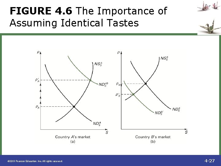
The Importance of Assuming Identical Tastes in the HO Model • See Figure 4. 6 • Initially, country A has a comparative advantage in good S due to lower autarky relative price and a lower supply curve (indicating natural comparative advantage). • Suppose that national tastes are different in that A’s citizens strongly prefer good S while B’s citizens do not. • As a result, A’s demand curve shifts upward while B’s demand shifts to the left. • Relative prices change such that B now has the comparative advantage in good S. © 2013 Pearson Education, Inc. All rights reserved. 4 -26

FIGURE 4. 6 The Importance of Assuming Identical Tastes © 2013 Pearson Education, Inc. All rights reserved. 4 -27

Some New HO Theorems • Rybczynski Theorem • Factor Price Equalization Theorem • Stolper-Samuelson Theorem © 2013 Pearson Education, Inc. All rights reserved. 4 -28

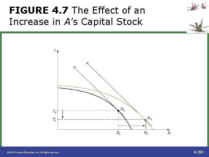
Rybczynski Theorem • At constant world prices, if a country experiences an increase in the supply of one factor, it will produce more of the product intensive in that factor and less of the other. • See Figure 4. 7 • Countries with high savings and investment rates will tend to produce and trade more capital-intensive goods. © 2013 Pearson Education, Inc. All rights reserved. 4 -29

FIGURE 4. 7 The Effect of an Increase in A’s Capital Stock © 2013 Pearson Education, Inc. All rights reserved. 4 -30

Factor Price Equalization Theorem • Given all the assumptions of the HO model, free international trade will lead to the international equalization of individual factor prices. • Country A is relatively capital-abundant and rent is low. With trade, the increase in demand for capital for producing exports raises rent. The opposite happens in country B. © 2013 Pearson Education, Inc. All rights reserved. 4 -31

Stolper-Samuelson Theorem • Free international trade benefits the abundant factor and harms the scarce factor. © 2013 Pearson Education, Inc. All rights reserved. 4 -32

Implications of Stolper. Samuelson Theorem • Some groups in society will oppose international trade. • Scarce factors will lobby government for trade protection. • Even though some in society lose, the country overall benefits from international trade relative to autarky. • A system of taxation and transfers could be developed to compensate the losers while leaving the gainers better off relative to autarky. See Global Insights 4. 2. © 2013 Pearson Education, Inc. All rights reserved. 4 -33