Chapter 4 The Heckscher Ohlin Model Copyright 2010

Chapter 4 The Heckscher. Ohlin Model Copyright © 2010 Pearson Addison-Wesley. All rights reserved.

Topics to be Covered • Heckscher-Ohlin model and assumptions • Factor endowment • Factor intensity • Trade equilibrium in the HO model • Rybczynski Theorem • Factor Price Equalization Theorem • Stolper-Samuelson Theorem Copyright © 2010 Pearson Addison-Wesley. All rights reserved. 4 -2

INTRODUCTION • What determines a country’s comparative advantage? • How does international trade affect the size of an economy’s various industries? • How does international trade affect the payments or returns to the factors of production? • How does international trade affect the distribution of income within a country? • To make sound business decisions it is necessary to understand what causes comparative advantage and how it can change over time Copyright © 2010 Pearson Addison-Wesley. All rights reserved. 4 -3

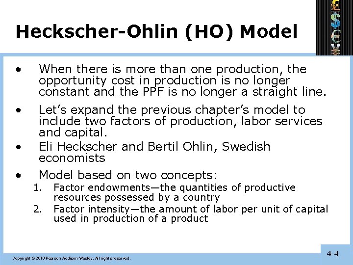
Heckscher-Ohlin (HO) Model • When there is more than one production, the opportunity cost in production is no longer constant and the PPF is no longer a straight line. • Let’s expand the previous chapter’s model to include two factors of production, labor services and capital. Eli Heckscher and Bertil Ohlin, Swedish economists Model based on two concepts: • • 1. 2. Factor endowments—the quantities of productive resources possessed by a country Factor intensity—the amount of labor per unit of capital used in production of a product Copyright © 2010 Pearson Addison-Wesley. All rights reserved. 4 -4

Assumptions of HO Model • Keep first 10 assumptions (in chapters 2 and 3) • Drop assumption 11 (labor is only resource) and 12 (constant returns to scale) • Add five new assumptions Copyright © 2010 Pearson Addison-Wesley. All rights reserved. 4 -5

Five New Assumptions • Assumption 13—Two resources, labor (L) and capital (K), and resource payments, wages for labor (W) and rent for capital (R) • Assumption 14—Identical technology in both countries; choice of production technique depends on factor prices (Note: this assumption rules out the classical basis for trade) Copyright © 2010 Pearson Addison-Wesley. All rights reserved. 4 -6

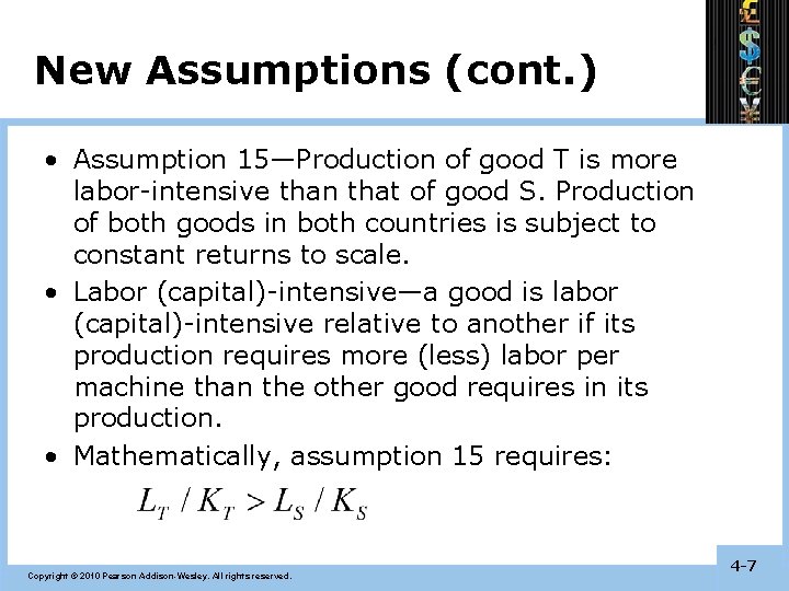
New Assumptions (cont. ) • Assumption 15—Production of good T is more labor-intensive than that of good S. Production of both goods in both countries is subject to constant returns to scale. • Labor (capital)-intensive—a good is labor (capital)-intensive relative to another if its production requires more (less) labor per machine than the other good requires in its production. • Mathematically, assumption 15 requires: Copyright © 2010 Pearson Addison-Wesley. All rights reserved. 4 -7

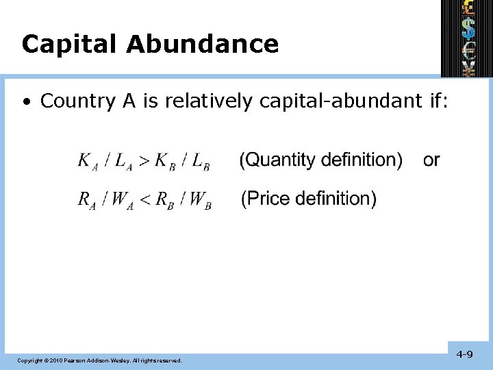
New Assumptions (cont. ) • Assumption 16—Country A is relatively capital-abundant while B is relatively laborabundant. • Two definitions of resource abundance: – Quantity definition – Price definition Copyright © 2010 Pearson Addison-Wesley. All rights reserved. 4 -8

Capital Abundance • Country A is relatively capital-abundant if: Copyright © 2010 Pearson Addison-Wesley. All rights reserved. 4 -9

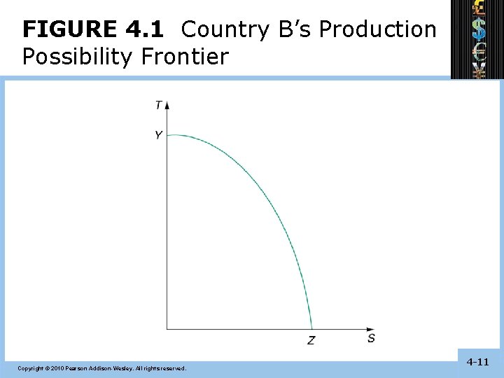
Production Possibility Frontier • Since the two goods differ in factor intensity in both countries, the PPFs of each country will exhibit increasing opportunity cost (i. e. , PPF will have a bowed out, nonlinear shape). International trade does not cause complete specialization • Because country B is labor-abundant and good T is labor-intensive, B’s PPF will lie primarily along (or biased toward) the Taxis (see Figure 4. 1). Copyright © 2010 Pearson Addison-Wesley. All rights reserved. 4 -10

FIGURE 4. 1 Country B’s Production Possibility Frontier Copyright © 2010 Pearson Addison-Wesley. All rights reserved. 4 -11

Assumption 17 • Tastes in the two countries are identical. That is, both countries have the same set of community indifference curves (CIC). • This assumption guarantees that a country’s comparative advantage is determined primarily by supply, not demand, factors. Copyright © 2010 Pearson Addison-Wesley. All rights reserved. 4 -12

Heckscher-Ohlin Theorem • A country will have comparative advantage in, and therefore will export, that good whose production is relatively intensive in the factor with which the country is relatively well-endowed. Copyright © 2010 Pearson Addison-Wesley. All rights reserved. 4 -13

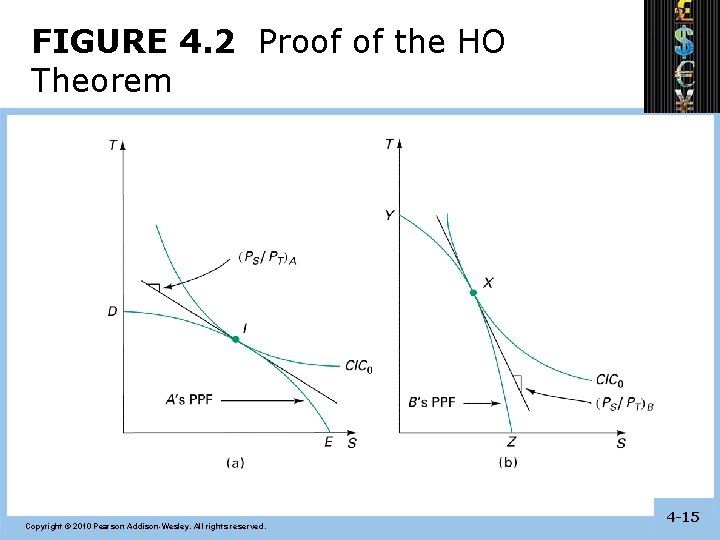
Graphical Proof of HO Theorem • Given different PPFs for the two countries and identical CICs, find autarky equilibrium points for both countries (see Figure 4. 2) • At the equilibrium point, the slope of each country’s PPF equals the pre-trade price ratio • Since (PS /PT )A < (PS /PT )B , then A(B) has comparative advantage in, and will export, good S(T) Copyright © 2010 Pearson Addison-Wesley. All rights reserved. 4 -14

FIGURE 4. 2 Proof of the HO Theorem Copyright © 2010 Pearson Addison-Wesley. All rights reserved. 4 -15

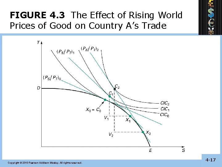
Effect of Rising World Price of Good S on Country A’s Trade • Refer to Figure 4. 3 below • Once trade begins, the price of S will rise (as represented by the three terms of trade or price lines) • As the price rises from (PS/PT)0 to (PS/PT)1 , A’s production point moves from X 0 to X 1. • With trade, A’s new consumption point is now C 1. • A’s trade triangle is V 1 C 1 X 1 where V 1 X 1 represents A’s exports and V 1 C 1 is A’s desired imports. • The terms of trade that will prevail once trade begins are determined by reciprocal demand. Copyright © 2010 Pearson Addison-Wesley. All rights reserved. 4 -16

FIGURE 4. 3 The Effect of Rising World Prices of Good on Country A’s Trade Copyright © 2010 Pearson Addison-Wesley. All rights reserved. 4 -17

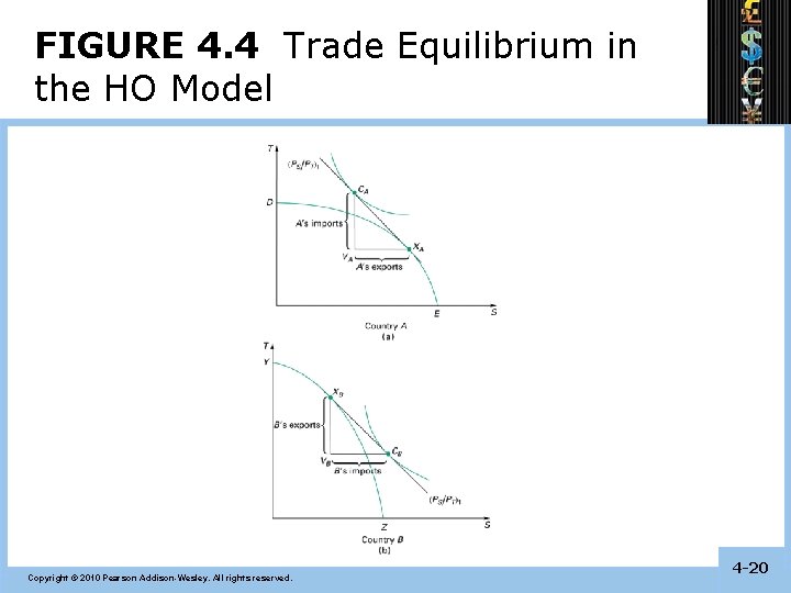
Trade Equilibrium in HO Model • Refer to Figure 4. 4 • Terms of trade are determined by reciprocal demand lie between the two countries’ pre-trade price ratios • Equilibrium production with trade exhibits incomplete specialization (due to increasing opportunity cost) • Equilibrium consumption with trade implies a rise in standard of living Copyright © 2010 Pearson Addison-Wesley. All rights reserved. 4 -18

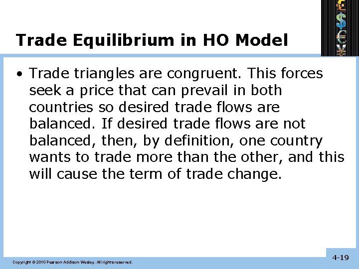
Trade Equilibrium in HO Model • Trade triangles are congruent. This forces seek a price that can prevail in both countries so desired trade flows are balanced. If desired trade flows are not balanced, then, by definition, one country wants to trade more than the other, and this will cause the term of trade change. Copyright © 2010 Pearson Addison-Wesley. All rights reserved. 4 -19

FIGURE 4. 4 Trade Equilibrium in the HO Model Copyright © 2010 Pearson Addison-Wesley. All rights reserved. 4 -20

Differences between Classical and HO Models • Complete specialization results in classical model, while incomplete specialization occurs in HO model. • In classical model, only demand conditions affect reciprocal demand. In HO model, reciprocal demand leads to equilibrium price via changes in both demand supply. • Autarky price in the classical model is determined only by supply conditions. In HO model, demand supply determine autarky price. Copyright © 2010 Pearson Addison-Wesley. All rights reserved. 4 -21

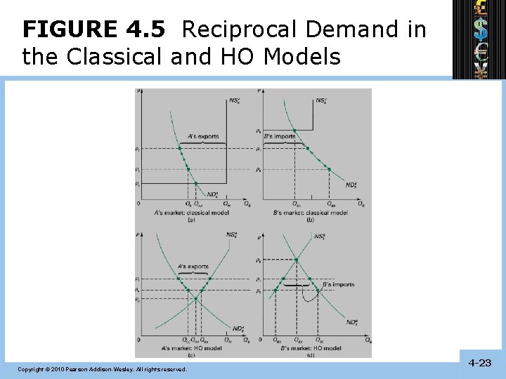
Reciprocal Demand in the Classical and HO Models • Refer to Figure 4. 5 the major difference between the tow diagrams is the, • The national supply curves differ in the two models. In the classical model, the national supply curve is horizontal (due to constant cost) up to the point of complete specialization, at which the curve becomes vertical. In the HO model, the curve is initially upward-sloping (due to increasing costs). • Autarky equilibrium is achieved where the national demand national supply curves intersect. Since the relative price PS/PT is lower in country A, then A has a comparative advantage in good S. Copyright © 2010 Pearson Addison-Wesley. All rights reserved. 4 -22

FIGURE 4. 5 Reciprocal Demand in the Classical and HO Models Copyright © 2010 Pearson Addison-Wesley. All rights reserved. 4 -23

Reciprocal Demand (Classical) • See Figures 4. 5 a and 4. 5 b. • When trade begins at a world price p 0, A’s production of S rises to its complete specialization level and A exports what it does not consume. In country B, production of S falls to zero and its imports of S increase. • Due to excess demand at p 0, the world price will rise and consumption in both countries will fall until the world markets attain equilibrium at new world price p 1. Copyright © 2010 Pearson Addison-Wesley. All rights reserved. 4 -24

Reciprocal Demand (HO Model) • See Figures 4. 5 c and 4. 5 d • Similar to the Classical model except in how the excess demand is eliminated. As the world price rises in response to the excess demand, consumption falls in both countries but supply also rises in both countries. Copyright © 2010 Pearson Addison-Wesley. All rights reserved. 4 -25

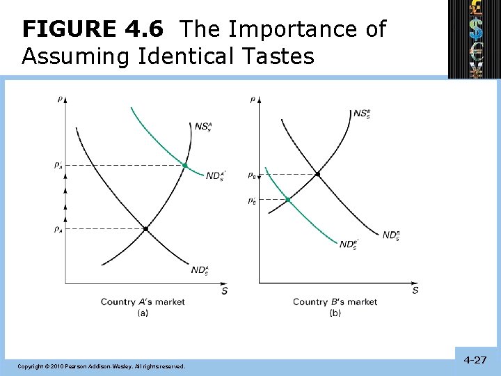
The Importance of Assuming Identical Tastes in the HO Model • See Figure 4. 6 • Initially, country A has a comparative advantage in good S due to lower autarky relative price and a lower supply curve (indicating natural comparative advantage). • Suppose that national tastes are different in that A’s citizens strongly prefer good S while B’s citizens do not. • As a result, A’s demand curve shifts upward while B’s demand shifts to the left. • Relative prices change such that B now has the comparative advantage in good S. Copyright © 2010 Pearson Addison-Wesley. All rights reserved. 4 -26

FIGURE 4. 6 The Importance of Assuming Identical Tastes Copyright © 2010 Pearson Addison-Wesley. All rights reserved. 4 -27

Extensions of the HO Theorem • Rybczynski Theorem • Factor Price Equalization Theorem • Stolper-Samuelson Theorem Copyright © 2010 Pearson Addison-Wesley. All rights reserved. 4 -28

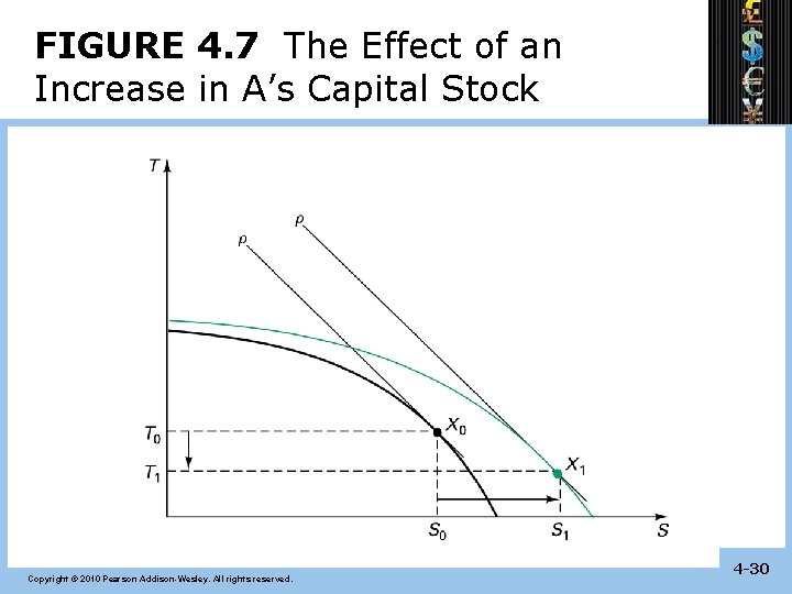
T. M Rybczynski Theorem 1955 • H-O mode offer several other important theories about economic behavior engaged in I trade, such as the effect of economic growth on trade and the impact that trade has on the distribution of income in the society. • At constant world prices, if a country experiences an increase in the supply of one factor, it will produce more of the product intensive in that factor and less of the other product. Copyright © 2010 Pearson Addison-Wesley. All rights reserved. 4 -29

FIGURE 4. 7 The Effect of an Increase in A’s Capital Stock Copyright © 2010 Pearson Addison-Wesley. All rights reserved. 4 -30

• The theory basically says that the on which a country grows has an impact on the production and trade mixes of that country. • Countries with low saving rates that invest little in new plant & equipment will tend to produce & trade goods with high labor content. • Countries with high saving & investment rates will tend to produce & trade more capital-intensive goods. Copyright © 2010 Pearson Addison-Wesley. All rights reserved. 4 -31

Factor Price Equalization • Unlike the Ricardian model, the Heckscher-Ohlin model predicts that input (factor) prices will be equalized among countries that trade. • Because relative output prices are equalized and because of the direct relationship between output prices and factor prices, factor prices are also equalized. • Trade increases the demand of goods produced by abundant factors, indirectly increasing the demand of the abundant factors themselves, raising the prices of the abundant factors across countries. Copyright © 2010 Pearson Addison-Wesley. All rights reserved. 4 -32

Factor Price Equalization (cont. ) • But factor prices are not really equal across countries. • The model assumes that trading countries produce the same goods, so that prices for those goods will equalize, but countries may produce different goods. • The model also assumes that trading countries have the same technology, but different technologies could affect the productivities of factors and therefore the wages/rates paid to these factors. • Factor equalization in HO model hold perfectly when tow main assumption exist, that is, no barriers to trade and identical technology. • Dan Ben David in 1993 has examined the effects of trade liberalization has affected income levels in different countries. Copyright © 2010 Pearson Addison-Wesley. All rights reserved. 4 -33

Factor Price Equalization Theorem • Given all the assumptions of the HO model, free international trade will lead to the international equalization of individual factor prices. • Country A is relatively capital-abundant and rent is low. With trade, the increase in demand for capital for producing exports raises rent. The opposite happens in country B. Copyright © 2010 Pearson Addison-Wesley. All rights reserved. 4 -34

Stolper-Samuelson Theorem • Free international trade benefits the abundant factor and harms the scarce factor. Copyright © 2010 Pearson Addison-Wesley. All rights reserved. 4 -35

Implications of Stolper. Samuelson Theorem • Some groups in society will oppose international trade. • Scarce factors will lobby government for trade protection. • Even though some in society lose, the country overall benefits from international trade relative to autarky. • A system of taxation and transfers could be developed to compensate the losers while leaving the gainers better off relative to autarky. Copyright © 2010 Pearson Addison-Wesley. All rights reserved. 4 -36