Causal Diagrams and the Identification of Causal Effects

Causal Diagrams and the Identification of Causal Effects Pearl J (2009). Causality. Chapter 3.

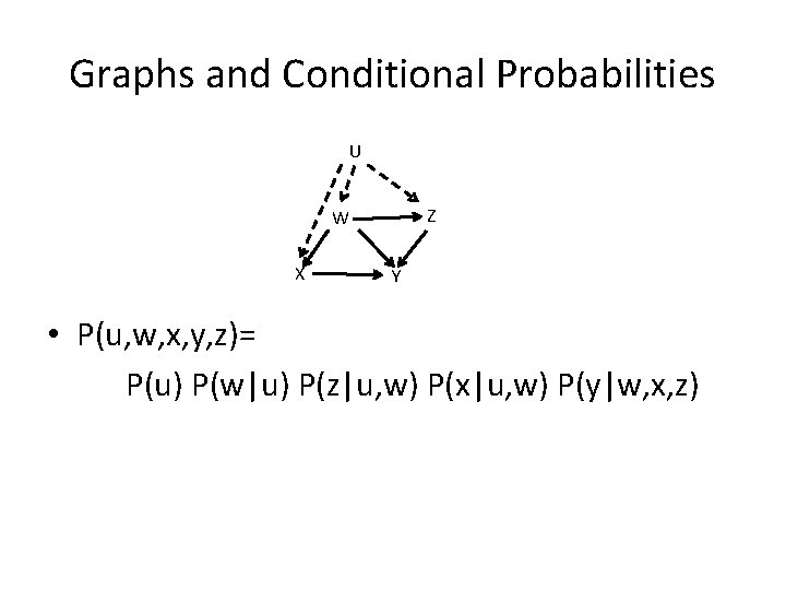
Graphs and Conditional Probabilities U Z W X Y • P(u, w, x, y, z)= P(u) P(w|u) P(z|u, w) P(x|u, w) P(y|w, x, z)

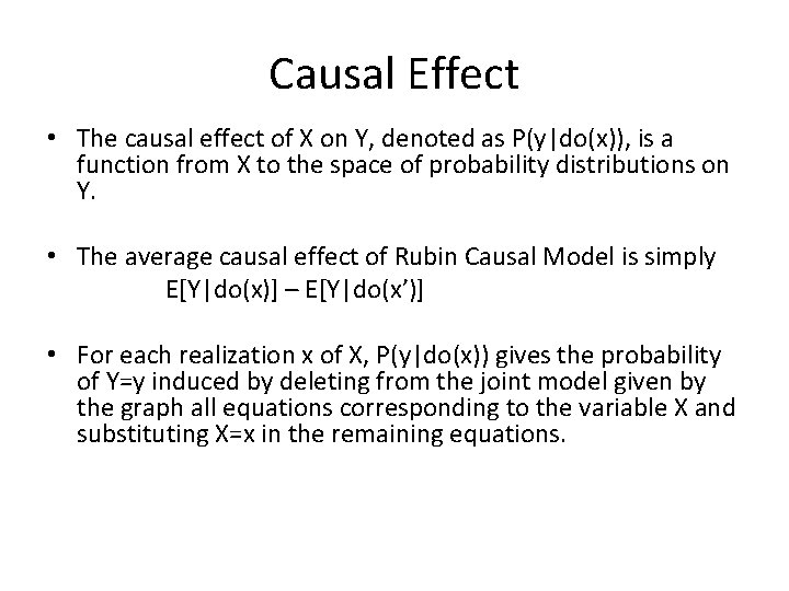
Causal Effect • The causal effect of X on Y, denoted as P(y|do(x)), is a function from X to the space of probability distributions on Y. • The average causal effect of Rubin Causal Model is simply E[Y|do(x)] – E[Y|do(x’)] • For each realization x of X, P(y|do(x)) gives the probability of Y=y induced by deleting from the joint model given by the graph all equations corresponding to the variable X and substituting X=x in the remaining equations.

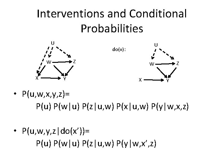
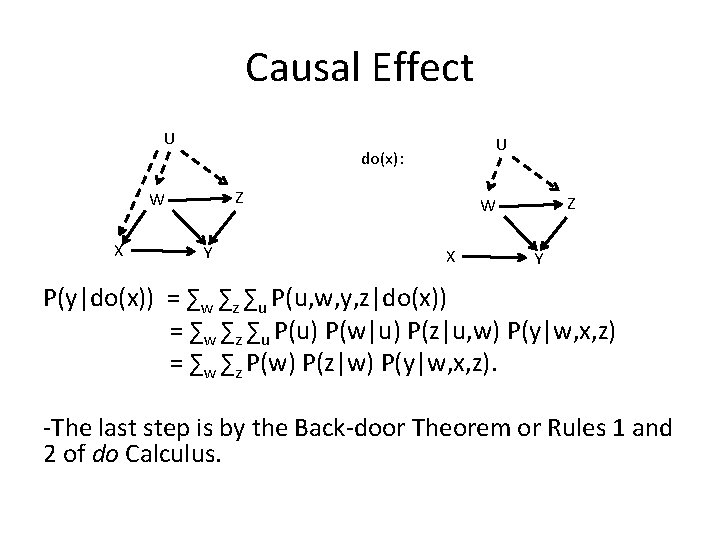
Interventions and Conditional Probabilities U do(x): Z W X U Y Z W X Y • P(u, w, x, y, z)= P(u) P(w|u) P(z|u, w) P(x|u, w) P(y|w, x, z) • P(u, w, y, z|do(x’))= P(u) P(w|u) P(z|u, w) P(y|w, x’, z)

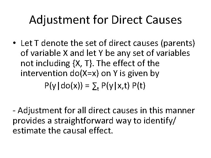
Adjustment for Direct Causes • Let T denote the set of direct causes (parents) of variable X and let Y be any set of variables not including {X, T}. The effect of the intervention do(X=x) on Y is given by P(y|do(x)) = ∑t P(y|x, t) P(t) - Adjustment for all direct causes in this manner provides a straightforward way to identify/ estimate the causal effect.

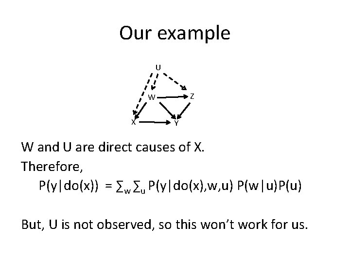
Our example U Z W X Y W and U are direct causes of X. Therefore, P(y|do(x)) = ∑w ∑u P(y|do(x), w, u) P(w|u)P(u) But, U is not observed, so this won’t work for us.

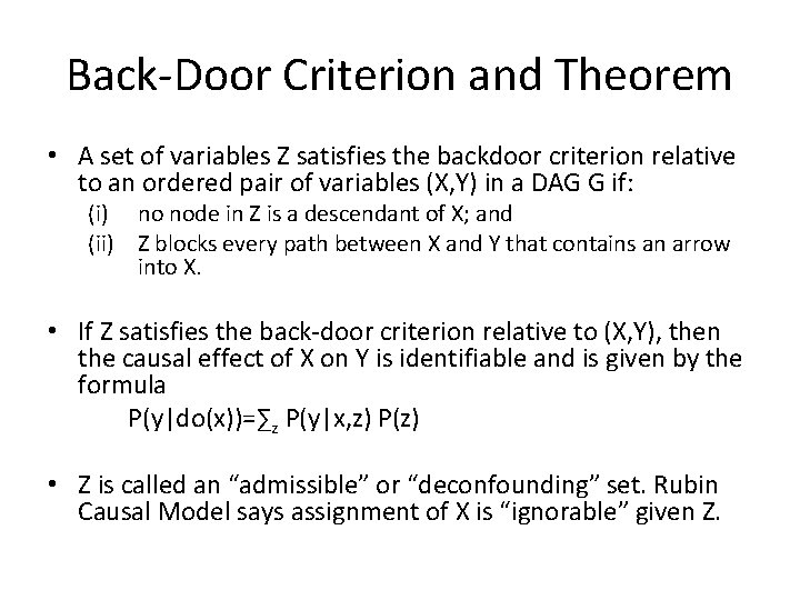
Back-Door Criterion and Theorem • A set of variables Z satisfies the backdoor criterion relative to an ordered pair of variables (X, Y) in a DAG G if: (i) no node in Z is a descendant of X; and (ii) Z blocks every path between X and Y that contains an arrow into X. • If Z satisfies the back-door criterion relative to (X, Y), then the causal effect of X on Y is identifiable and is given by the formula P(y|do(x))=∑z P(y|x, z) P(z) • Z is called an “admissible” or “deconfounding” set. Rubin Causal Model says assignment of X is “ignorable” given Z.

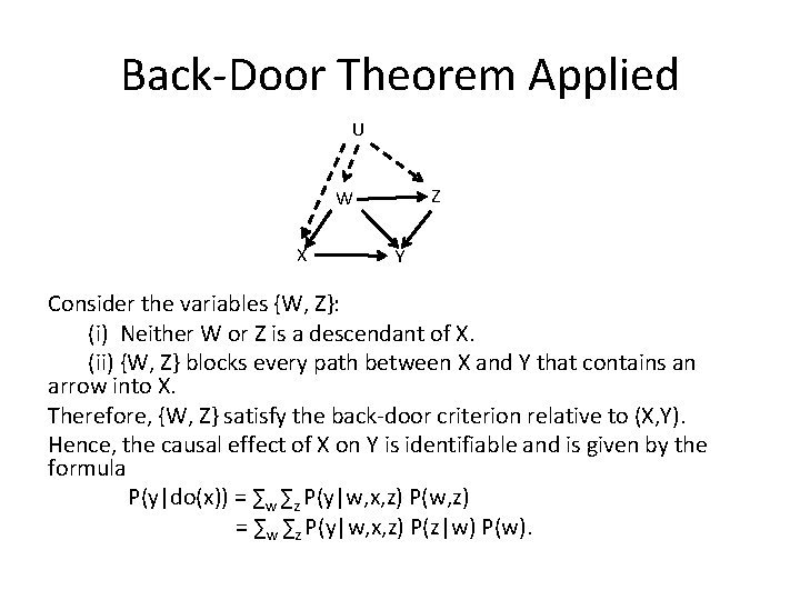
Back-Door Theorem Applied U Z W X Y Consider the variables {W, Z}: (i) Neither W or Z is a descendant of X. (ii) {W, Z} blocks every path between X and Y that contains an arrow into X. Therefore, {W, Z} satisfy the back-door criterion relative to (X, Y). Hence, the causal effect of X on Y is identifiable and is given by the formula P(y|do(x)) = ∑w ∑z P(y|w, x, z) P(w, z) = ∑w ∑z P(y|w, x, z) P(z|w) P(w).

Causal Effect U do(x): Z W X U Y Z W X Y P(y|do(x)) = ∑w ∑z ∑u P(u, w, y, z|do(x)) = ∑w ∑z ∑u P(u) P(w|u) P(z|u, w) P(y|w, x, z) = ∑w ∑z P(w) P(z|w) P(y|w, x, z). -The last step is by the Back-door Theorem or Rules 1 and 2 of do Calculus.

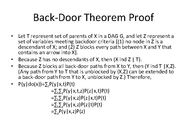
Back-Door Theorem Proof • Let T represent set of parents of X in a DAG G, and let Z represent a set of variables meeting backdoor criteria [(1) no node in Z is a descendant of X; and (2) Z blocks every path between X and Y that contains an arrow into X]. • Because Z has no descendants of X, then (X ind Z | T). • Because Z blocks all back-door paths from X to Y, then (Y ind T |X, Z). (Any path from Y to T that is unblocked by {X, Z} can be extended to a back-door path from Y to X, unblocked by Z. ) Therefore, • P(y|do(x))=∑t. P(y|x, t)P(t) =∑t∑z. P(y|x, t, z)P(z|x, t)P(t) =∑t∑z. P(y|x, z)P(z|t)P(t) =∑z. P(y|x, z)P(z)

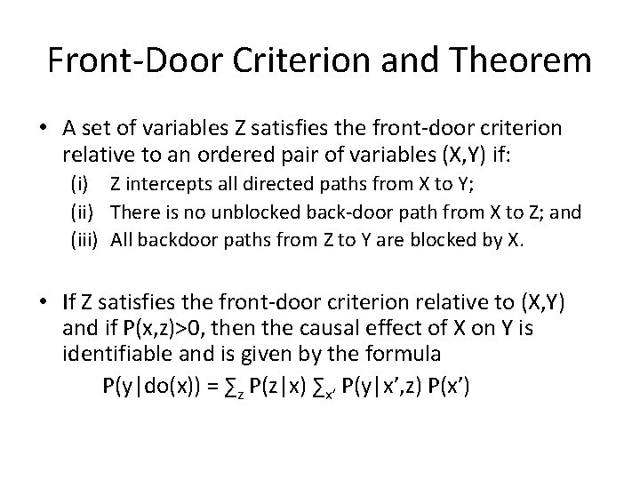
Front-Door Criterion and Theorem • A set of variables Z satisfies the front-door criterion relative to an ordered pair of variables (X, Y) if: (i) Z intercepts all directed paths from X to Y; (ii) There is no unblocked back-door path from X to Z; and (iii) All backdoor paths from Z to Y are blocked by X. • If Z satisfies the front-door criterion relative to (X, Y) and if P(x, z)>0, then the causal effect of X on Y is identifiable and is given by the formula P(y|do(x)) = ∑z P(z|x) ∑x’ P(y|x’, z) P(x’)

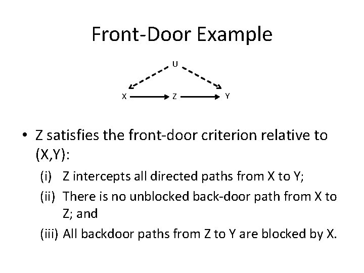
Front-Door Example U X Z Y • Z satisfies the front-door criterion relative to (X, Y): (i) Z intercepts all directed paths from X to Y; (ii) There is no unblocked back-door path from X to Z; and (iii) All backdoor paths from Z to Y are blocked by X.

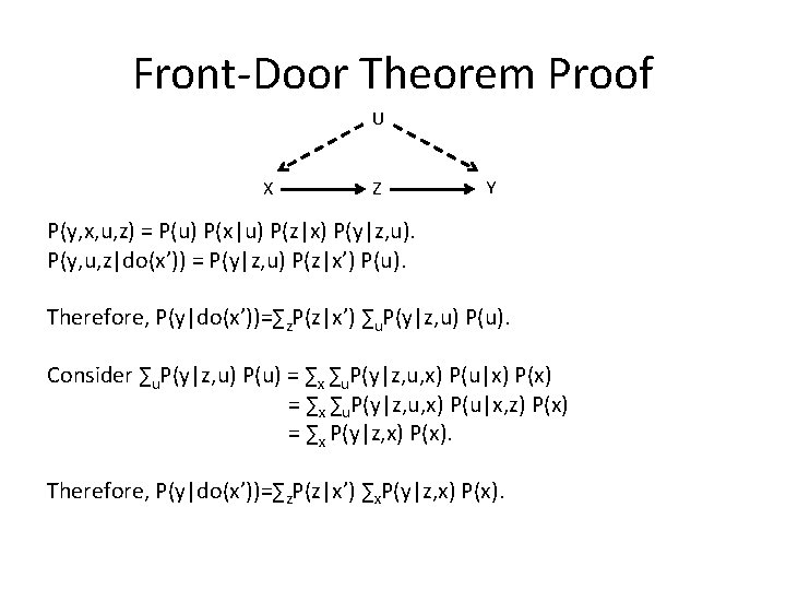
Front-Door Theorem Proof U X Z Y P(y, x, u, z) = P(u) P(x|u) P(z|x) P(y|z, u). P(y, u, z|do(x’)) = P(y|z, u) P(z|x’) P(u). Therefore, P(y|do(x’))=∑z. P(z|x’) ∑u. P(y|z, u) P(u). Consider ∑u. P(y|z, u) P(u) = ∑x ∑u. P(y|z, u, x) P(u|x) P(x) = ∑x ∑u. P(y|z, u, x) P(u|x, z) P(x) = ∑x P(y|z, x) P(x). Therefore, P(y|do(x’))=∑z. P(z|x’) ∑x. P(y|z, x) P(x).

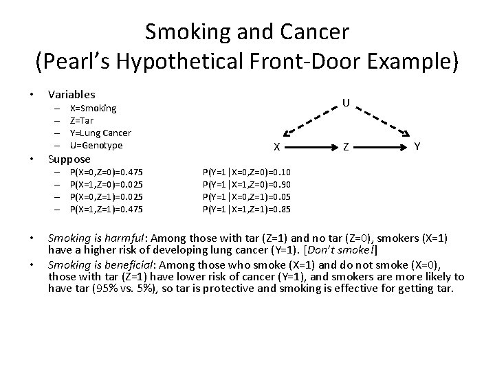
Smoking and Cancer (Pearl’s Hypothetical Front-Door Example) • Variables – – • Suppose – – • • X=Smoking Z=Tar Y=Lung Cancer U=Genotype P(X=0, Z=0)=0. 475 P(X=1, Z=0)=0. 025 P(X=0, Z=1)=0. 025 P(X=1, Z=1)=0. 475 U X Z Y P(Y=1|X=0, Z=0)=0. 10 P(Y=1|X=1, Z=0)=0. 90 P(Y=1|X=0, Z=1)=0. 05 P(Y=1|X=1, Z=1)=0. 85 Smoking is harmful: Among those with tar (Z=1) and no tar (Z=0), smokers (X=1) have a higher risk of developing lung cancer (Y=1). [Don’t smoke!] Smoking is beneficial: Among those who smoke (X=1) and do not smoke (X=0), those with tar (Z=1) have lower risk of cancer (Y=1), and smokers are more likely to have tar (95% vs. 5%), so tar is protective and smoking is effective for getting tar.

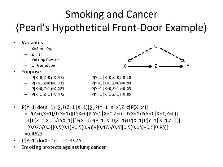
Smoking and Cancer (Pearl’s Hypothetical Front-Door Example) • Variables – – • Suppose – – • • • X=Smoking Z=Tar Y=Lung Cancer U=Genotype P(X=0, Z=0)=0. 475 P(X=1, Z=0)=0. 025 P(X=0, Z=1)=0. 025 P(X=1, Z=1)=0. 475 U X Z P(Y=1|X=0, Z=0)=0. 10 P(Y=1|X=1, Z=0)=0. 90 P(Y=1|X=0, Z=1)=0. 05 P(Y=1|X=1, Z=1)=0. 85 P(Y=1|do(X=1)=∑z. P(Z=1|X=1)[∑x’P(Y=1|X=x’, Z=z)P(X=x’)] =[P(Z=0, X=1)/P(X=1)][P(X=0)P(Y=1|X=0, Z=0)+P(X=1)P(Y=1|X=1, Z=0)] +[P(Z=1, X=1)/P(X=1)][P(X=0)P(Y=1|X=0, Z=1)+P(X=1)P(Y=1|X=1, Z=1)] =[0. 025/0. 5][0. 5(0. 1)+0. 5(0. 9)]+[0. 475/0. 5][0. 5(0. 05)+0. 5(0. 85)] =0. 4525 P(Y=1|do(X=0)=…. =0. 4975 Smoking protects against lung cancer Y

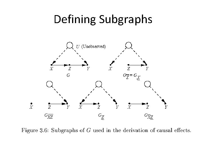
Defining Subgraphs

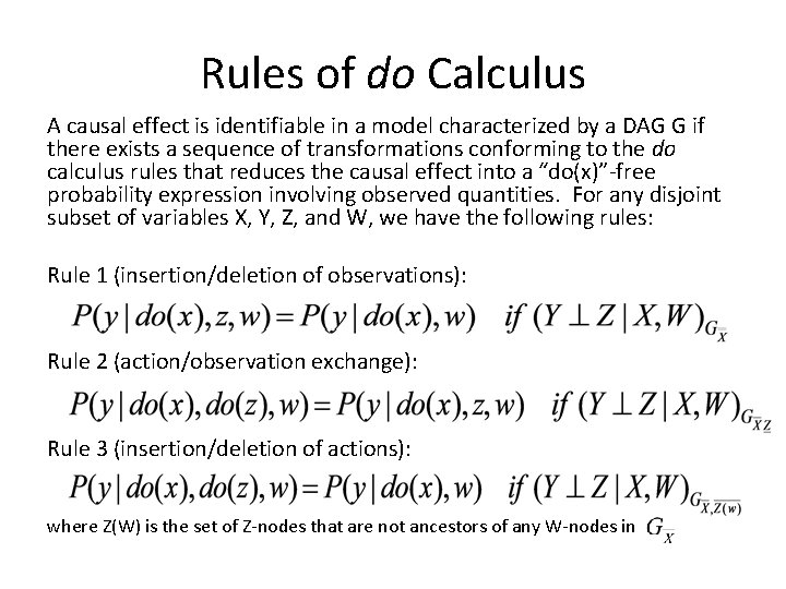
Rules of do Calculus A causal effect is identifiable in a model characterized by a DAG G if there exists a sequence of transformations conforming to the do calculus rules that reduces the causal effect into a “do(x)”-free probability expression involving observed quantities. For any disjoint subset of variables X, Y, Z, and W, we have the following rules: Rule 1 (insertion/deletion of observations): Rule 2 (action/observation exchange): Rule 3 (insertion/deletion of actions): where Z(W) is the set of Z-nodes that are not ancestors of any W-nodes in

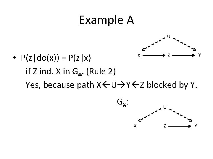
Example A U • P(z|do(x)) = P(z|x) if Z ind. X in GX. (Rule 2) Yes, because path X U Y Z blocked by Y. X G X: Z U X Z Y Y

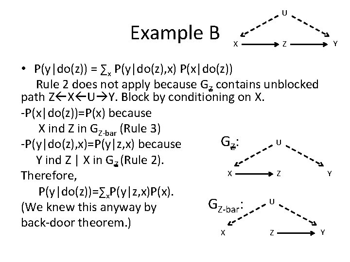
U Example B X • P(y|do(z)) = ∑x P(y|do(z), x) P(x|do(z)) Rule 2 does not apply because GZ contains unblocked path Z X U Y. Block by conditioning on X. -P(x|do(z))=P(x) because X ind Z in GZ-bar (Rule 3) U G Z: -P(y|do(z), x)=P(y|z, x) because Y ind Z | X in GZ (Rule 2). X Z Therefore, P(y|do(z))=∑x. P(y|z, x)P(x). U GZ-bar: (We knew this anyway by back-door theorem. ) X Y Z Z Y Y

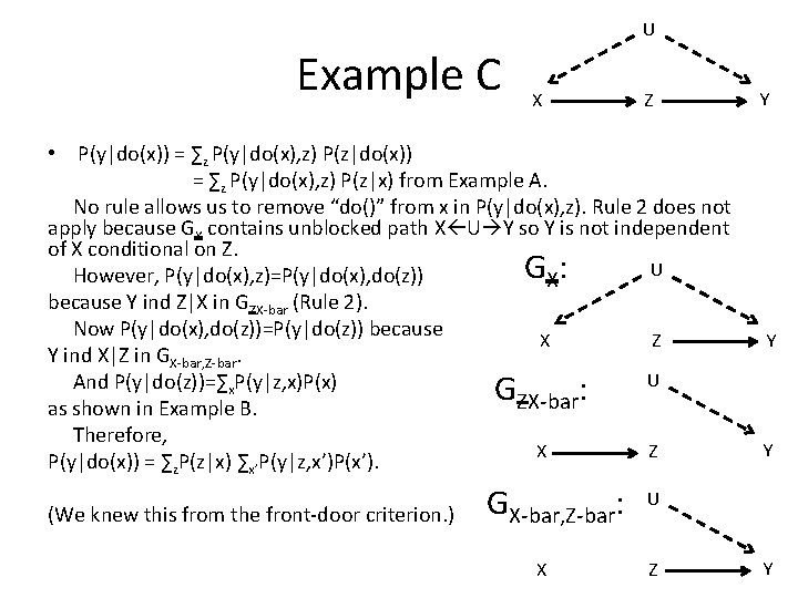
U Example C X Z • P(y|do(x)) = ∑z P(y|do(x), z) P(z|x) from Example A. No rule allows us to remove “do()” from x in P(y|do(x), z). Rule 2 does not apply because GX contains unblocked path X U Y so Y is not independent of X conditional on Z. U G X: However, P(y|do(x), z)=P(y|do(x), do(z)) because Y ind Z|X in GZX-bar (Rule 2). Now P(y|do(x), do(z))=P(y|do(z)) because X Z Y ind X|Z in GX-bar, Z-bar. U And P(y|do(z))=∑x. P(y|z, x)P(x) G : ZX-bar as shown in Example B. Therefore, X Z P(y|do(x)) = ∑z. P(z|x) ∑x’P(y|z, x’)P(x’). (We knew this from the front-door criterion. ) GX-bar, Z-bar: X Y Y Y U Z Y

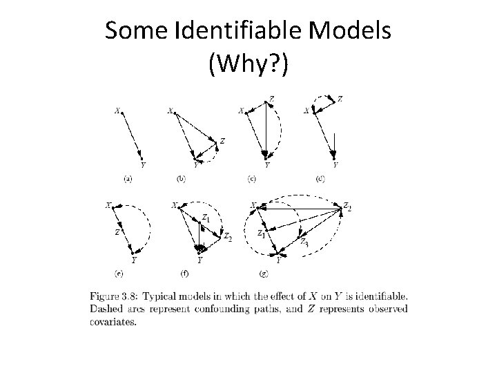
Some Identifiable Models (Why? )

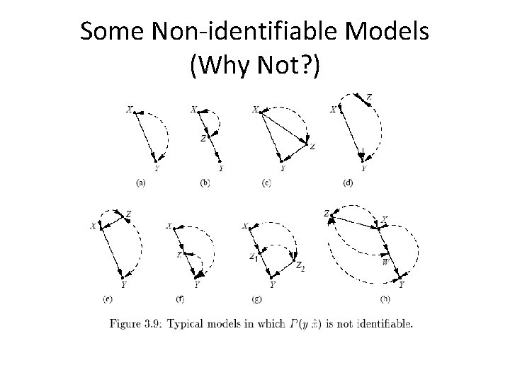
Some Non-identifiable Models (Why Not? )

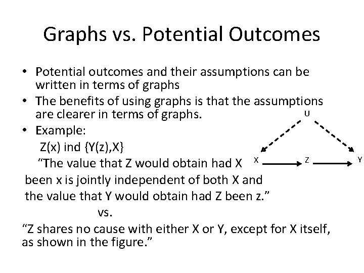
Graphs vs. Potential Outcomes • Potential outcomes and their assumptions can be written in terms of graphs • The benefits of using graphs is that the assumptions U are clearer in terms of graphs. • Example: Z(x) ind {Y(z), X} Z “The value that Z would obtain had X X been x is jointly independent of both X and the value that Y would obtain had Z been z. ” vs. “Z shares no cause with either X or Y, except for X itself, as shown in the figure. ” Y

Graphs vs. Potential Outcomes • “The thought of having to express, defend, and manage formidable counterfactual relationships of this type may explain why the enterprise of causal inference is currently viewed with such awe and despair among rank -and-file epidemiologists and statisticians – and why most economists and social scientists continue to use structural equations instead of the potential-outcomes alternatives. ” -Pearl

Graphs vs. Potential Outcomes • Pearl is particularly critical of the conditional ignorability assumption commonly made: {Y(0), Y(1)} ind X | Z. • “Strong ignorability…is a convenient syntactic tool for manipulating counterfactual formulas, as well as a convenient way of formally assuming admissibility (of Z) without having to justify it. ” • “However, …hardly anyone knows how to apply it in practice, because the counterfactual variables Y(0) and Y(1) are unobservable, and scientific knowledge is not stored in a form that allows reliable judgment about conditional independence of counterfactuals. ”

Graphs vs. Potential Outcomes • “On the other hand, the algebraic machinery offered by the potential-outcome notation, once a problem is properly formalized, can be quite powerful in refining assumptions, deriving probabilities of counterfactuals, and verifying whether conclusions follow from premises. ” -Pearl • Potential outcomes notation allows things to be written in terms of probabilities – no need for do(x) operations. • e. g. , {Y(0), Y(1)} ind X|Z implies P(Y(x)=y)=∑z. P(Y(x)=y|z)P(z) =∑z. P(Y(x)=y|x, z)P(z) (by ignorability) =∑z. P(Y=y|x, z)P(z) (by consistency: X=x implies Y(x)=Y) which is what we get from the back-door-theorem.

Graphs vs. Potential Outcomes Imbens and Rubin (2015): “Pearl advocates a different approach to causality. Pearl combines aspects of structural equations models and path diagrams. In this approach, assumptions underlying causal statements are coded as missing links in the path diagrams. Mathematical methods are then used to infer, from these path diagrams, which causal effects can be inferred from the data, and which cannot… Pearl’s work is interesting and many find his arguments that path diagrams are a natural and convenient way to express assumptions about causal structures appealing. In our own work, perhaps influenced by the type of examples arising in social and medical sciences, we have not found this approach to aid drawing of causal inferences, and we do not discuss it further in this text. ”