Behavioral Analysis 4 inferential statistics 5 Statistical test
 inferential statistics –第 5章 統計的仮説検定 • Statistical test of")
行動計量分析 Behavioral Analysis • 第 4回 推測統計学の考え方(2) inferential statistics –第 5章 統計的仮説検定 • Statistical test of hypothesis –母数の区間推定 interval estimation https: //stattrek. com/hypothesis-test/mean. aspx 1

記述統計学と推測統計学 Descriptive Statistics vs Inferential Statistics Descriptive Statistics 目の前の 多数のデータ Data of many objects in front of you 多数データの 数学的要約・記述 Summarize and describe simply Inferential Statistics (仮想的) 母集団 (imaginary) population (無作為)抽出 sampling 標本集団 のデータ Data of samples 確率的推測・記述 Stochastic Inference 少数データの 数学的要約・記述 Summarize the smaller samples 2
 Two major problems in Inference Statistics • 統計的推定 statistical estimation, inference Ø")
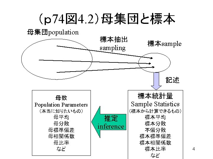
4.2 推測統計の分類(p 72) Two major problems in Inference Statistics • 統計的推定 statistical estimation, inference Ø サンプル値から計算した統計量の実現値をもとに,母集 団の確率分布を決めるパラメータ(母数)を推定 Statistical estimation: Estimate the Parameter Value governing the Population Distribution, based on the function of the sample values. We usually use the representative value of the samples as the function to estimate the (population) parameter. Ø 標本中学生のテスト結果の平均値から,日本の中学生全 体の同じテストの平均値を推測する Estimate the average mark of all Japanese high school students, based on the mark of the sample students. Ø 中学生全体の平均は 60点ぐらいだろう(点推定)Point estimation Ø 中学生全体の平均は 50点から70点ぐらいだろう(区間推定) 3 Interval Estimation
 We want to know the average height of 22 yr")
点推定 point estimation • 22歳日本人男性の平均身長は?(母数:母平均) We want to know the average height of 22 yr old Japanese Men. (Parameter = ave. of the population) • 10人の 22歳男性を標本抽出し, 身長計測値を得る Measure height of 10 sample men. (Sample values) • 10個の計測値から,標本の平均値を計算する(169. 3) Sample mean was calculated from the sample values • 標本の平均値を用い,22歳日本人男性の平均身長を推測す る Estimate the Population mean from the sample mean. height <- c(165. 2, 175. 9, 161. 7, 174. 2, 172. 1, 163. 3, 170. 9, 170. 6, 168. 4, 171. 3) height [1] 165. 2 175. 9 161. 7 174. 2 172. 1 163. 3 170. 9 170. 6 168. 4 171. 3 mean(height) [1] 169. 36 5
がどのぐらい真値に近いかはよくわか らない。 We cannot tell how the")
点推定量の性質 Characteristics of the estimator • たまたま取ってきたひと組みの標本から計算した 値(推定値)がどのぐらい真値に近いかはよくわか らない。 We cannot tell how the estimates (obtained value of the estimator) calculated from the one samples in front of you, is near to the true population parameter. • さまざまな標本から同じ計算方法で推定値を求 める場合のその推定量の統計的な性質を考える。 We discuss the characteristics of the distribution of the estimator. (Repeat sampling many times) 6
不偏性:標本を何回も取り直して推定量を計算すると、 その平均値が真値に一致する Unbiasedness : Average of the estimators of")
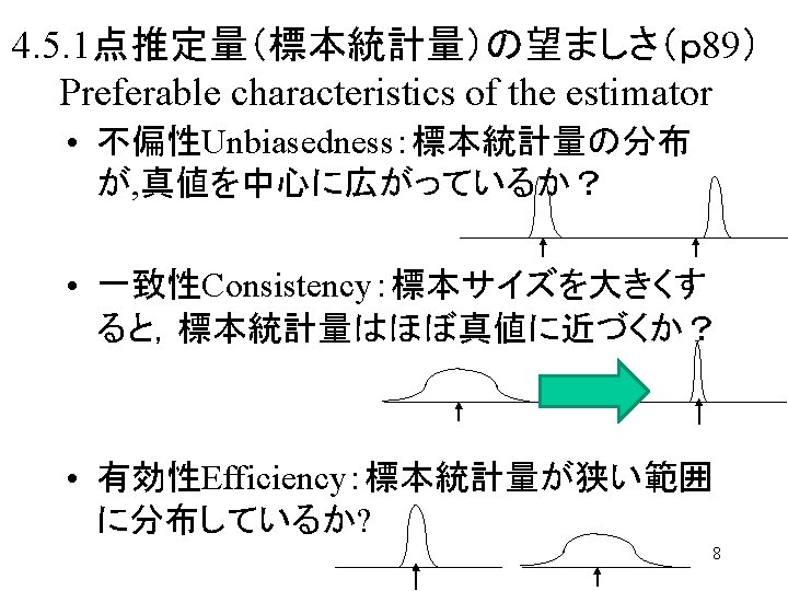
点推定量の性質 Characteristics of the estimator 1)不偏性:標本を何回も取り直して推定量を計算すると、 その平均値が真値に一致する Unbiasedness : Average of the estimators of the repeated samplings coincident to the true parameter value. 2)一致性:標本の数を十分大きくするとその一組の標本 からの推定量が真値をとる確率が1に近づく Consistency: If sample size becomes larger, the estimator distribution converges to the real value. 3)有効性:推定量の分散が、他の方法で計算した推定 量の分散よりも小さい Efficiency:Variance of the estimator is smaller than 7 that of any other estimator.
 Unbiased estimator of the population variance (population mean is unknown) • 11")
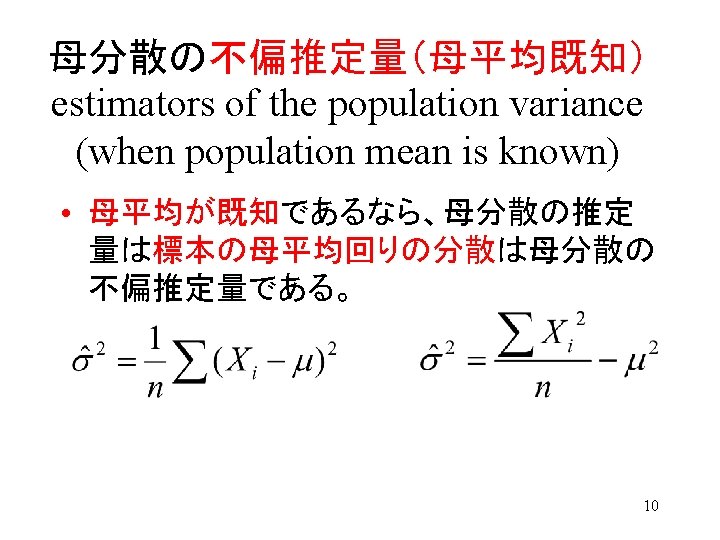
母分散の不偏推定量(母平均未知) Unbiased estimator of the population variance (population mean is unknown) • 11

母平均周りの分散と,標本平均周りの分散 Variance around population mean & Variance around sample mean # Define new function to calculate variance centered around ”m” varp <- function(x, m) { smplvar <- mean((x-m*rep(1, length(x)))*(x-m*rep(1, length(x)))) smplvar } #母集団分布を仮定する(正規分布) Monte Carlo Simulaton of sample variances varpopm<-numeric(length=10000); varsmpm<-numeric(length=10000) for(i in 1: 10000){ sampleset <- rnorm(n=10, mean=50, sd=10) #generate sampleset varpopm [i] <- varp(sampleset, 50) # store Variance 1 varsmpm [i] <-varp(sampleset, mean(sampleset)) # store Variance 2 } hist(varsmpm, freq=FALSE, border="blue") hist(varpopm, freq=FALSE, border="red", add=TRUE) curve(dchisq(x/10, 10)/10, add=TRUE) mean(varpopm); var(varpopm) # Variance 1 (unbiased =100) mean(varsmpm); var(varsmpm) # Variance 2 (biased= 90=100/10*9) hist(varsmpm*10/9, freq=FALSE, border="green", add=TRUE) # Variance 2 adjusted 12

母平均周りの分散と,標本平均周りの分散 Variance around population mean & Variance around sample mean Variance around population mean: unbiased Theoretical chi-square Distribution: unbiased Variance around sample mean divided by n: biased (smaller) Variance around sample mean divided by n-1: Unbiased Estimator 13

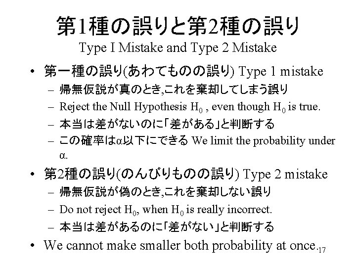
統計的仮説検定 Test of Statistical Hypothesis 1 母集団に対する帰無仮説と対立仮説を設定する Settle H 0: Null Hypothesis and H 1: Alternate Hypothesis 2.検定統計量を選ぶ Choose Statistics (function of sample value) 3.有意水準の値を決める Decide Level of Significance 4.データから, 検定統計量の実現値を求める Calculate the value of the Statistics based on the sample values 5.検定統計量の実現値を棄却域と比較する Compare the value of statistics referring the "reject area" (1)実現値⊂棄却域→帰無仮説を棄却,対立仮説を採択 Statistics value ⊂ reject area, -> Reject H 0, Approve H 1 (2)実現値⊂棄却域→帰無仮説を棄却しない(判断保留) Statistics value ⊂ reject area, -> Cannot reject H 0 14 (no active conclusion)
 • H 0:日本人の平均体重は 50 kgである(μ=μ 0")
帰無仮説と対立仮説 Null Hypothesis and Alternate Hypothesis 帰無仮説(null hypothesis) • H 0:日本人の平均体重は 50 kgである(μ=μ 0 or δ=μ-μ 0=0) Population Mean of Japanese weight is 50 kg. 対立仮説(alternative hypothesis) • H 1: 日本人平均体重は 50 kgではない (μ≠μ 0 or δ=μ-μ 0≠ 0) Population Mean of Japanese weight is not 50 kg. 両側検定 Two-side test • H 1: 日本人平均体重は 50 kgより大きい (μ>μ 0 or δ=μ-μ 0>0) Population Mean of Japanese weight is larger than 50 kg. 片側検定 One-side test 15

検定統計量と棄却域・採択域 Test Statistics, reject area and approve area • 検定のために用いる標本統計量 Test Statistics – 帰無仮説が成り立つ場合は (母数の真値を用いて) 標 本統計量が従う確率分布がわかり, 確率を計算できる – When Null Hypothesis (concerning the population parameter value) is true, we can calculate the distribution of the Statistics (based on it). • 帰無仮説の下で非常に生じにくい(ある小さな確率α以下で しか生じない)値の範囲を「棄却域」という. • Reject Area: the statistics value sits in the area, with particularly small probability α, such as 0. 05 or 0. 01. • それ以外の領域を「採択域」という Approved Area: else Approved 採択域 Approved 棄却域(両側) Reject Area(both side) 棄却域(片側) Reject Area(one side) 16

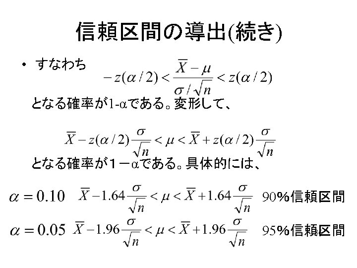
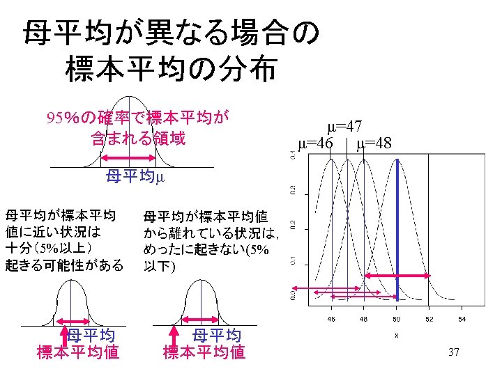
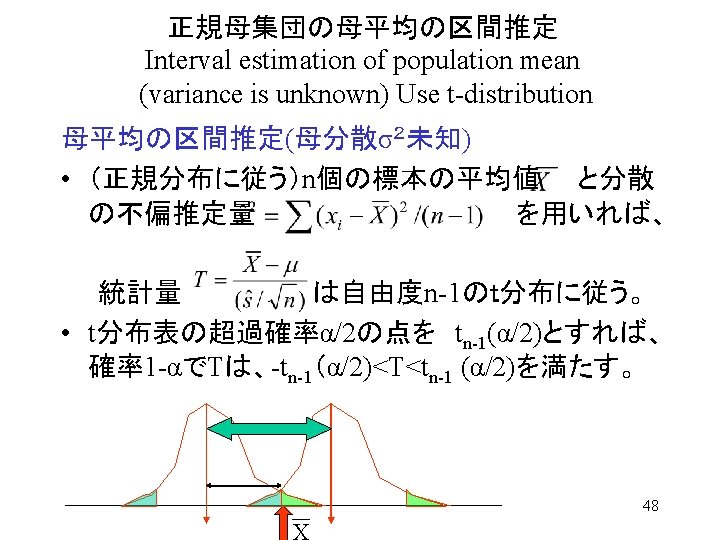
区間推定 Interval Estimation • 母数の真値が のとき、ある統計量の確率分布を求めて「有意水準α以 下の確率でしか出現しない領域」を棄却域とした。 Reject area was set, where the statistics sits in with probability smaller than α, if parameter equals to (if Ho is true). • 標本を何回もとり直した場合,統計量の実現値がこの棄却域に入るような (標本値が得られる)確率は、α/2以下である。 Probability of that Statistics value sits either of the reject area must be less than α/2. • 母数の真値 が統計量実現値から大きく離れていたような状況は,せ いぜい確率 α. でしか起こらないはず! (本当はおかしい解釈.母数は動 かないもの) Parameter may locate near to the realized value of the statistics , with 1 -α 信頼区間 probability of 1 -α. Confidence Interval 統計量の 確率 α/2 θ 0 Distribution of Statistics for given parameter value 統計量の実現値 Realized Statistics 19

区間推定 Interval Estimation 統計量の分布が左右非対称な場合には特に注意すること Be careful when distribution of statistics is asymmetric! 1 -α 信頼区間 Confidence Interval 統計量の 確率 α/2 θ 0 Distribution of Statistics for given parameter value 統計量の実現値 Realized Statistics 20

統計量の確率分布を知ることが重要 distribution of parameter estimator • Parameter estimates takes various values depending on the realized value of the samples: It is also a probabilistic variables (parameter estimator) 例)標本の実 現値を均等に 用いる単純平 均値という「統 計量」 母集団分布 Population Distiribution + 推定量の計算方法 Def. Statistics ↓ 推定量の確率分布 Distribution of Estimator 21
, are theoretically derived • Population Distribution 母集団の性質を決める,個々の事 象が発生する確率分布や平均値など(母数)が与えられた とき,")
Some distribution of estimators (statistics), are theoretically derived • Population Distribution 母集団の性質を決める,個々の事 象が発生する確率分布や平均値など(母数)が与えられた とき, • Distribution of a Statistics (defined by a function) 標本値から計算される統計量の確率分布を計算したい • Analytical relationship are derived in some cases. 一般にこの計算は面倒だが,いくつかは解析的に計算式 がわかっている. 母集団の分布 要約値(統計量) Population の確率分布 Distribution of the 母数 Estimator (statistics) 法則性, 計算式 Patameter Definition of statistics 22 (function)
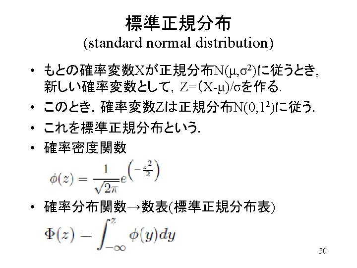
 確率密度関数 平均と分散 Reproduction Theorem Why Normal Distribution is frequently used? 正規分布の再生性 ・Reproduction 正規分布変数の和は")
正規分布(Normal Distribution) 確率密度関数 平均と分散 Reproduction Theorem Why Normal Distribution is frequently used? 正規分布の再生性 ・Reproduction 正規分布変数の和は 正規分布に従う ・Central Limit Theory 23

正規分布に従う母集団の 母数に関する仮説検定 Parameter Test for the Normal Distributed Population • Mean Variance • Pop var. known Normal dist. χ2 dist. • Pop var. unknown t-dist. χ2 dist. • 母分散未知で未知の母平均の同一性の検定 t Equality of two unknown means under unknown var. • 未知の母分散の同一性の検定:F Equality of unknown variances 24
 based on Normal Distributed Variables 正規分布する母集団からの標本値から計算する 統計量(正規確率変数の関数)の確率分布 • 25")
Distribution of a Statistics (function) based on Normal Distributed Variables 正規分布する母集団からの標本値から計算する 統計量(正規確率変数の関数)の確率分布 • 25

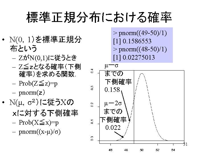
正規分布変数の平均値の分布 Sample mean of Nornmal Ditributed Variables. • • 母平均μ母分散σ2の母集団 大きさnの標本を取り出す 標本平均を計算 「標本平均」は母集団分布よ りも中央に集まった分布に • 実際正規母集団 N(50, 10)か らn=100のサンプルをとる smpmean<- numeric(length=10000) for(i in 1: 10000){ smpset <- rnorm(n=100, mean=50, sd=10) smpmean[i]<- mean(smpset) } curve(dnorm(x, mean=50, sd=1), from=20, to=80) curve(dnorm(x, mean=50, sd=10), add = TRUE) hist(smpmean, freq=FALSE, add=TRUE) • 標本平均は正規分布に従う. 26
 母平均の検定(母分散既知) Z-test:Test of population mean when population variance is known. 27")
1) 母平均の検定(母分散既知) Z-test:Test of population mean when population variance is known. 27

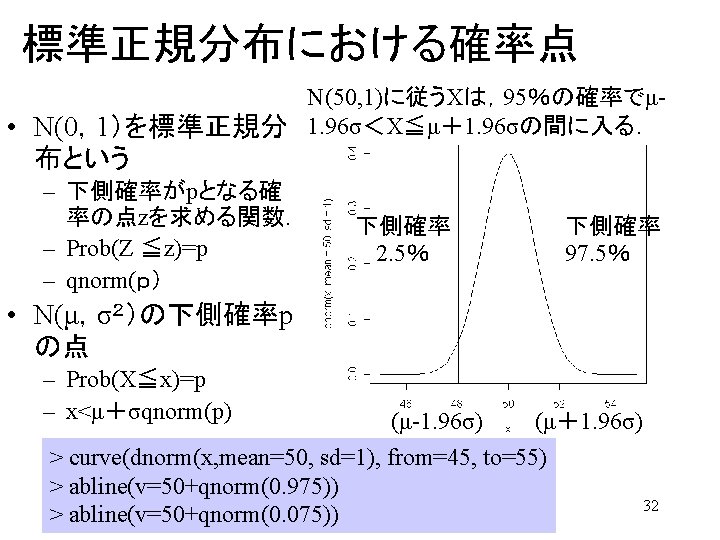
Test of population mean when population variance is known. Z-test In a z-test, the sample is assumed to be normally distributed. A z-score is calculated with population parameters such as “population mean” and “population standard deviation” and is used to validate a hypothesis that the sample drawn belongs to the same population. Null: Sample mean is same as the population mean Alternate: Sample mean is not same as the population mean The statistics used for this hypothesis testing is called z-statistic, the score for which is calculated as z = (x — μ) / (σ / √n), where x= sample mean μ = population mean σ / √n = population standard deviation If the test statistic is lower than the critical value, accept the hypothesis or else reject the hypothesis 28

29
=1. 645 Z(0. 05/2)=1. 96 Z(0. 01/2)=2. 575 38")
Z(0. 10/2)=1. 645 Z(0. 05/2)=1. 96 Z(0. 01/2)=2. 575 38
母平均の検定(母分散未知) t-test:Test of population mean when population variance is unknown. T-test Like a z-test,")
2)母平均の検定(母分散未知) t-test:Test of population mean when population variance is unknown. T-test Like a z-test, a t-test also assumes a normal distribution of the sample. A t-test is used when the population parameters (mean and standard deviation) are not known. There are three versions of t-test 1. Independent samples t-test which compares mean for two groups 2. Paired sample t-test which compares means from the same group at different times 3. One sample t-test which tests the mean of a single group against a known mean. 40
 42")
t分布表 (Student’s t distribution) 42
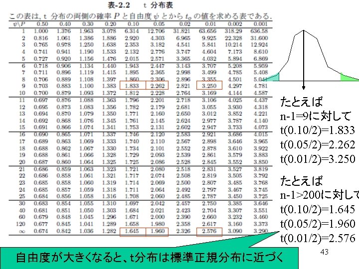

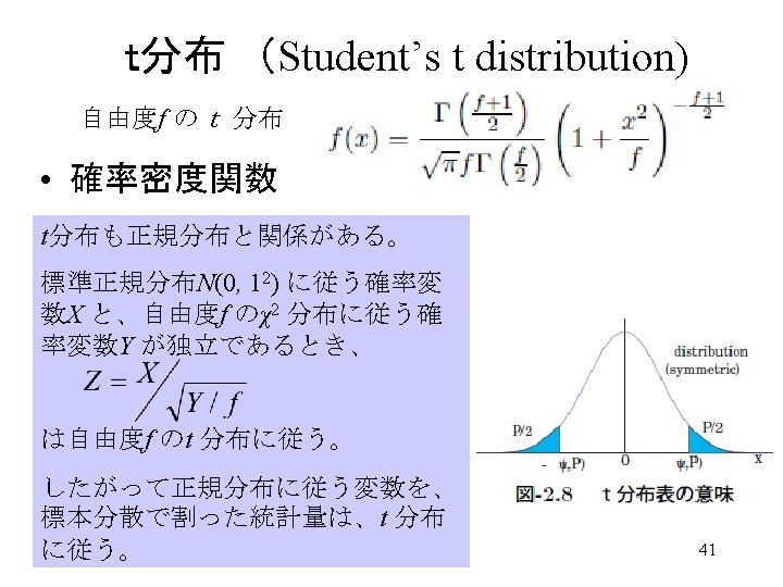
正規母集団からの標本値の確率分布 Mean and Variance of one sample set from one population 正規分布母集団 Normal Distributed Population Sample set 不偏分散推定量 Unbiased Variance 不偏標準偏差による標準化 Standardized by Unbiased Estimator t分布に従う。 Standardized Y obeys Student’s t distribution. 45
 sd. X<-numeric(length=1000)")
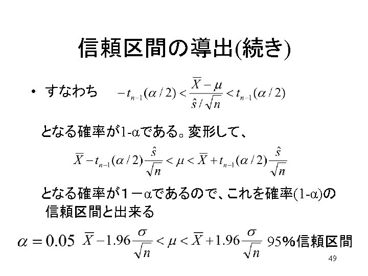
不偏分散推定量で標準化したサンプル値の分布 Distribution of Value after standardization by unbiased SD estimator smp. X<-numeric(length=1000) sd. X<-numeric(length=1000) smp. Y<- numeric(length=1000) m 1<-0; sg 1<-sqrt(10) #Monte Carlo Simulation for(i in 1: 1000){ X <- rnorm(n=10, mean=m 1, sd=sg 1) smp. X[i] <- (X[1]-mean(X)) sd. X[i]<-sd(X) smp. Y[i]<- smp. X[i]/sd. X[i] } #Distribution of Y variable curve(dnorm(x, mean=0, sd=1), from=-3. 5, to=3. 5) hist(smp. Y, freq=FALSE, add=TRUE) curve(dt(x, 9), col = "violet", add = TRUE) Normal-distribution t-distribution 46

47
母分散の検定(母平均既知) Test of Population variance (mean is known) Chi-Square Test for sample variance 3)母分散の検定(母平均未知)")
3)母分散の検定(母平均既知) Test of Population variance (mean is known) Chi-Square Test for sample variance 3)母分散の検定(母平均未知) Test of Population variance (mean is unknown) Chi-Square Test for unbiased variance estimator 50
 52")
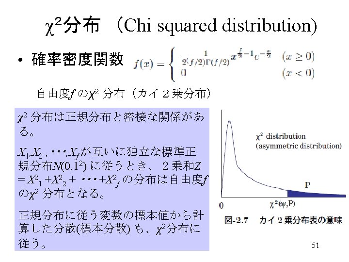
χ2分布表 (Chi squared distribution) 52
 4. 4. 5 var. A<-numeric(length=10000);")
正規母集団からの分散推定量はカイ 2乗分布 Estimator of Variances from Normal Distributed samples #母集団分布を仮定する(正規分布) 4. 4. 5 var. A<-numeric(length=10000); var. B<-numeric(length=10000) var. AB <-numeric(length=10000); na<-20; nb<-10 for(i in 1: 10000){ sampleset. A <- rnorm(n=na+1, mean=0, sd=1) #generate sample na+1 sampleset. B <- rnorm(n=nb+1, mean=0, sd=1) #generate sample nb+1 var. A [i] <- var(sampleset. A) # store Variance A var. B [i] <-var(sampleset. B) # store Variance B } curve(dchisq(x*na, na)*na, 0, 3. 5) hist(var. A, freq=FALSE, border="blue" , add=TRUE) curve(dchisq(x*nb, nb)*nb, add=TRUE) hist(var. B, freq=FALSE, border="red", add=TRUE) mean(var. A); var(var. A) # Variance A mean(var. B); var(var. B) # Variance B # The result shows chi-sq distribution 53
母分散の検定(母平均既知) Test of Population variance (mean is known) 54")
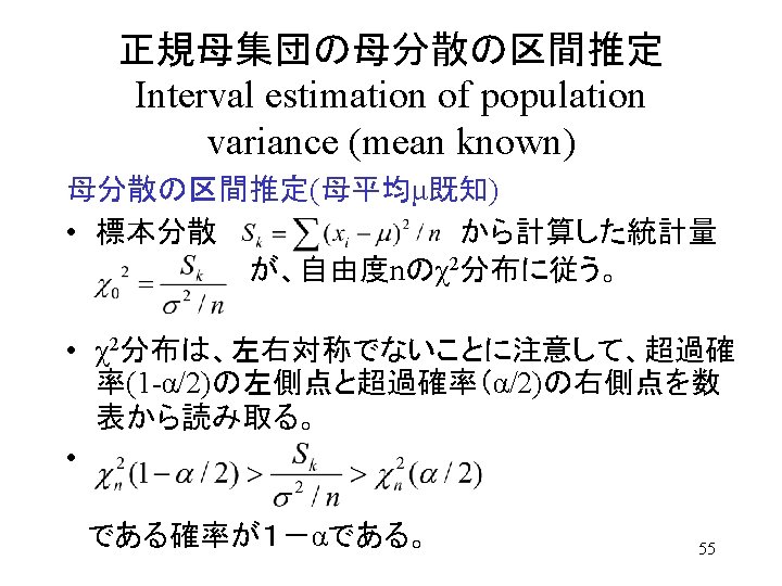
3)母分散の検定(母平均既知) Test of Population variance (mean is known) 54

56
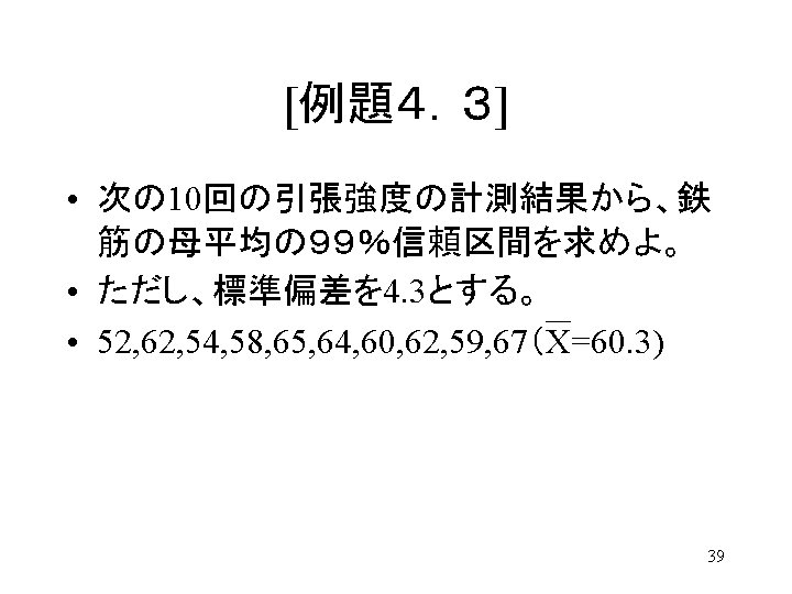
![[例題4.4] • 次の 10回の引張強度の計測結果から、鉄 筋の母分散の99%信頼区間を求めよ。 • ただし、母平均をμ=65とする。 • 52, 62, 54, 58, 65, 64,](http://slidetodoc.com/presentation_image_h/849bb6e423e6a709eee01294cd490aa1/image-58.jpg "[例題4.4] • 次の 10回の引張強度の計測結果から、鉄 筋の母分散の99%信頼区間を求めよ。 • ただし、母平均をμ=65とする。 • 52, 62, 54, 58, 65, 64,")
[例題4.4] • 次の 10回の引張強度の計測結果から、鉄 筋の母分散の99%信頼区間を求めよ。 • ただし、母平均をμ=65とする。 • 52, 62, 54, 58, 65, 64, 60, 62, 59, 67(X=60. 3) # Define function of variance centered around ”m” varp <- function(x, m) { mean((x-m*rep(1, length(x)))*(x-m*rep(1, length(x)))) } XX <- c(52, 62, 54, 58, 65, 64, 60, 62, 59, 67) Sk <-varp(XX, 65) # If mu is unknown, Variance around sample mean divided by n-1! Su <- varp(XX, mean(XX))*length(XX)/(length(XX)-1) 58 Sv <-var(XX)
![> Sk; qch 25; qch 975 [1] 42. 3 [1] 3. 246973 [1] 20.](http://slidetodoc.com/presentation_image_h/849bb6e423e6a709eee01294cd490aa1/image-59.jpg "> Sk; qch 25; qch 975 [1] 42. 3 [1] 3. 246973 [1] 20.")
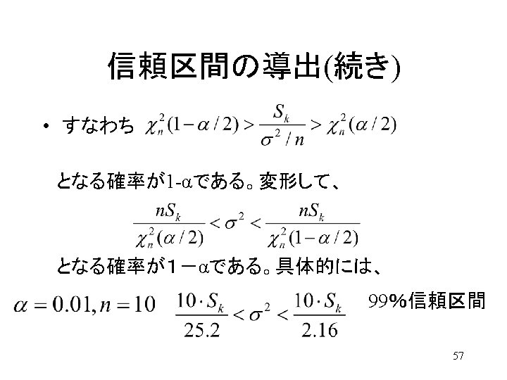
> Sk; qch 25; qch 975 [1] 42. 3 [1] 3. 246973 [1] 20. 48318 > Sk*10/qch 25 [1] 130. 2752 > Sk*10/qch 975 [1] 20. 65109 # Define d. Sk function give chisq # density to Sk for correct vp and n) d. Sk <-function(S, vp, n){ dchisq((S*n/vp), n) } # Draw graph of d. Sk qch 25=qchisq(0. 025, 10) qch 975=qchisq(0. 975, 10) Sk; qch 25; qch 975 Sk*10/qch 25 Sk*10/qch 975 curve(d. Sk(x, Sk/qch 975*10, 10)*qch 975, 0, 200) curve(d. Sk(x, Sk/qch 25*10, 10)*qch 25, 0, 200 , add=TRUE) curve(d. Sk(x, Sk/10*10, 10)*10, 0, 200, add=TRUE) abline(h=0) abline(v=Sk) 59

# Define d. Su function give chisq > Su ; qch 25; qch 975 # density to Su for correct vp and n) [1] 22. 45556 d. Su <-function(Su, vp, n){ [1] 2. 700389 [1] 19. 02277 dchisq((Su*n/vp), n-1) > Su*(10 -1)/qch 25 } [1] 74. 84106 # Draw graph of d. Su > Su*(10 -1)/qch 975 [1] 10. 62411 qch 25=qchisq(0. 025, 9); qch 975=qchisq(0. 975, 9) ; qch 975 Su ; qch 25; qch 975 Su*(10 -1)/qch 25 Su*(10 -1)/qch 975 curve(d. Su(x, Su/qch 975*9, 9)*qch 975, 0, 120) curve(d. Su(x, Su/qch 25*9, 9)*qch 25, 0, 120 , add=TRUE) curve(d. Su(x, Su/10*9, 9)*10, 1, 120, add=TRUE) abline(h=0) abline(v=Su) 62
2グループの分散の同一性の検定 (母平均は未知) F-test for equality of variance of two sample groups. ANOVA, also known")
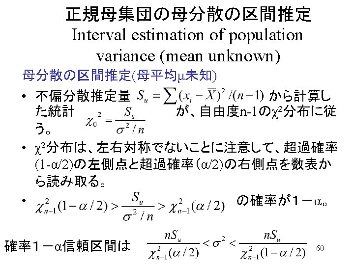
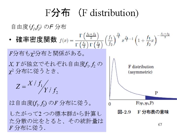
4)2グループの分散の同一性の検定 (母平均は未知) F-test for equality of variance of two sample groups. ANOVA, also known as analysis of variance, is used to compare multiple (three or more) samples with a single test. Use F-distribution 63

同じ正規母集団からの 2つの分散とその比 Variances of two sample sets from one population 正規分布母集団 Normal Distributed Population Sample set B Sample set A 不偏分散推定量 Unbiased Variance 分散の比 Ratio of Variances 分散の比は、F分布に従う。 Ratio of the two variances obeys F distribution. 64
 4. 4. 5 var. A<-numeric(length=10000);")
正規母集団からの分散推定量はカイ 2乗分布 Estimator of Variances from Normal Distributed samples #母集団分布を仮定する(正規分布) 4. 4. 5 var. A<-numeric(length=10000); var. B<-numeric(length=10000) var. AB <-numeric(length=10000); na<-20; nb<-10 for(i in 1: 10000){ sampleset. A <- rnorm(n=na+1, mean=0, sd=1) #generate sampleset. B <- rnorm(n=nb+1, mean=0, sd=1) #generate sampleset var. A [i] <- var(sampleset. A) # store Variance A var. B [i] <-var(sampleset. B) # store Variance B var. AB[i] <- var(sampleset. A) / var(sampleset. B) } curve(dchisq(x*na, na)*na, 0, 3. 5) hist(var. A, freq=FALSE, border="blue" , add=TRUE) curve(dchisq(x*nb, nb)*nb, add=TRUE) hist(var. B, freq=FALSE, border="red", add=TRUE) mean(var. A); var(var. A) # Variance A mean(var. B); var(var. B) # Variance B # The result shows chi-sq distribution 65

同じ母集団からの 2つの分散の比はF分布 Variances of two sample sets from one population #Distribution of the ratio of the two variances calculated from samples mean(var. AB); var(var. AB) # Ratio of two Variances hist(var. AB, freq=FALSE, border="green") #histogram of the ratio of two variances curve(df(x, na, nb), add=TRUE) # theoretical distribution (F with na and nb DF) 同じ母集団からの 2つの標 本から分散を計算し、その 比をとったものは、F分布に 従う。 Ratio of the two variances of two sample sets from one population obeys F distribution. 66
 68")
F分布表 (F distribution) 68
- Slides: 68