Inferential Statistics Chapter 7 Inferential Statistics Making inferences

Inferential Statistics Chapter 7 Inferential Statistics: Making inferences about populations based on samples

Hypothesis Testing A systematic procedure for deciding whether the results of a research study (using a sample) supports a hypothesis that applies to a population (probabilistic conclusion) Hypothesis: A predictions tested in a research study based on informal observation or theory e. g. , Concrete words are remembered better than Abstract Theory: a set of principles that attempts to explain one or more facts, relationships, or events usually gives rise to various specific hypotheses that can be tested in research studies e. g. , Dual-coding Theory: Concrete 2 codes & Abstract 1 code

The Core Logic of Hypothesis Testing • Researchers must spell out predictions in advance (A priori) to conclude that their hypothesis was supported. • Establish the p-value (a priori) of getting our experimental results if our hypothesis was not true. • Researchers attempt to answer these questions: • What is the probability of getting our research results if the opposite of what we predicted were true? • If it is highly unlikely that we would get our research results if the opposite of what we are predicting were true:

Research Hypothesis (H 1): Those chosen are more intelligent µ 1 1 > µ 2 µ 1 has a higher mean intelligence than µ 2 Null Hypothesis (H 0): Those chosen are not more intelligent µ 1 = µ 2 µ 1 does not have higher mean intelligence than µ 2

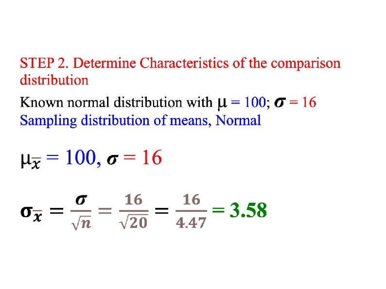
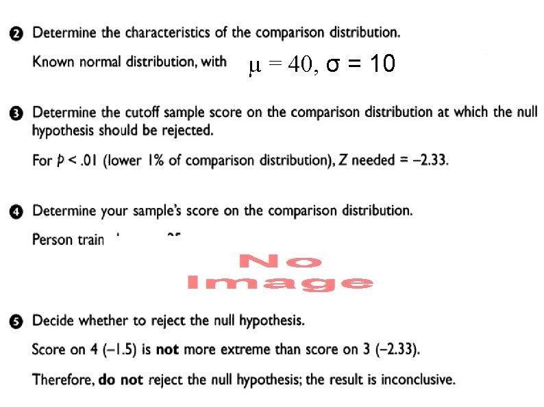
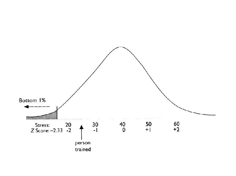
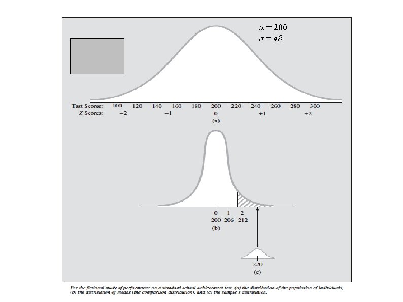
STEP 2. Define Characteristics of the comparison distribution Known normal distribution with µ = 100; σ = 16

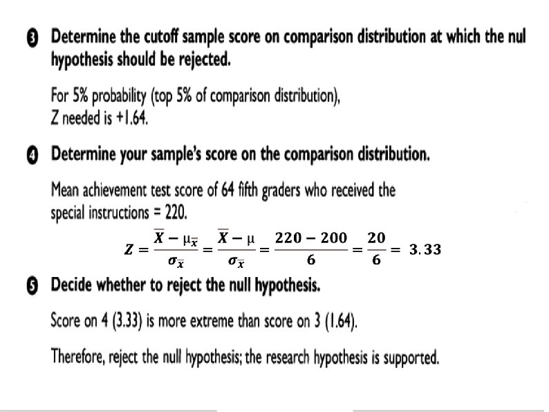
STEP 3. Determine cutoff (chosen a priori) sample scores on the comparison distribution at which the null hypothesis is rejected ( p =. 05) p <. 05 or top 5% : (50% -5% = 45%) Z = 1. 64

STEP 3. Cutoff sample score on the comparison distribution at which the null hypothesis is rejected. p =. 05 indicates that assuming the H 0 is true there is a 5% probability of obtaining a score as extreme, or more extreme, than our study prediction. This indicates our study prediction is unlikely when the starting assumption (H 0) is true. If the p-value is low enough (<. 05) we reject our starting assumption or the null hypothesis

Probability and Significance p <. 05 This result is so extreme or so unusual (top 5%) that chance cannot explain it Null Hypothesis Significance Testing (NHST)

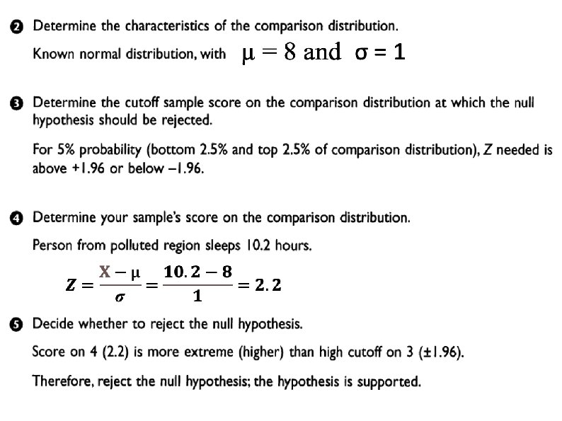
5. Compare the scores obtained in Step 3 and 4 to decide whether to reject the null hypothesis: Score on Step 4 (Z = 2. 5) is higher than score on Step 3 (Z = 1. 64) Conclusion: Reject H 0; H 1 is supported

Implications of Rejecting or Failing to Reject the Null Hypothesis When you reject the null hypothesis all you are saying is that your results support the research hypothesis. The results never prove the research hypothesis or show that your hypothesis is true. Research studies and their results are based on the probability or chance of getting your result if the null hypothesis were true. When you fail to reject or accept the null hypothesis, you do not say that the results support the null hypothesis. You say that the results are not statistically significant, or that the results are inconclusive. We are basing research on probabilities, and the fact that we did not find a result in this study does not mean that the null hypothesis is true.

Sampling Distribution of Means Sampling distribution of means: Distribution of means of all possible samples of a given size drawn randomly from the population.

Characteristics of a Sampling distribution of Means The mean or expected value of the mean of the sampling distribution of means is about the same as the mean of the original population of individuals (true for all sampling distributions of means). The spread of the sampling distribution of means is less than the spread of the distribution of the population of individuals (true for all samplings distributions of means). Shape of sampling distribution of means is approximately normal (true for most sampling distributions of means).

Expected Value of the Mean of a sampling Distribution of Means The mean or expected value of the mean of a sampling distribution of means (µx ) of samples of a given size from a particular population It is the same as the mean of the population of individuals. (µx ) = µ Because the selection process is random and because we are taking a very large number of samples, eventually the high means and the low means perfectly balance each other out.

σ2 and σ of the Sampling Distribution of Means If each sample has n = 1, the sampling distribution of means is the same as the population of individuals When sample size is 2 or more, variance/ of the sampling distribution of means is always smaller than the variance of the population. This is because the probability of getting two or more extreme cases in the same direction is less than getting just one. The more cases in each sample, the smaller the variation.

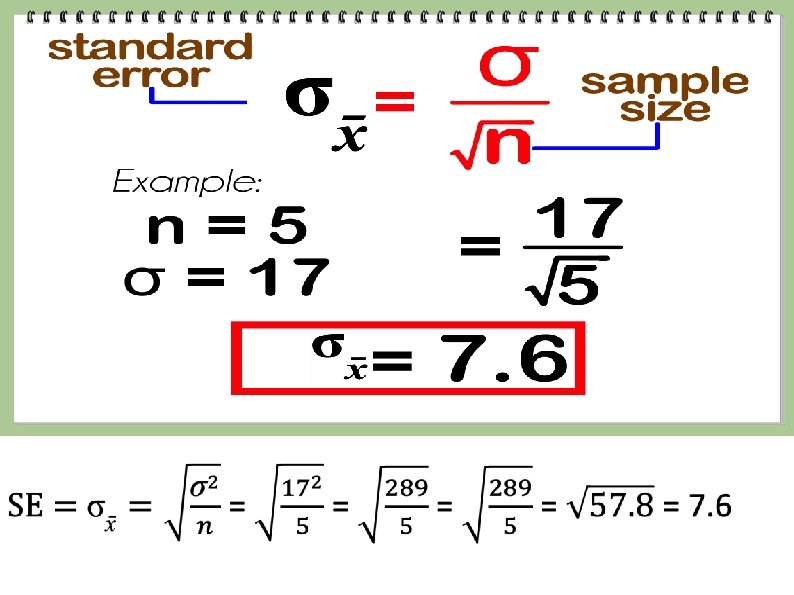
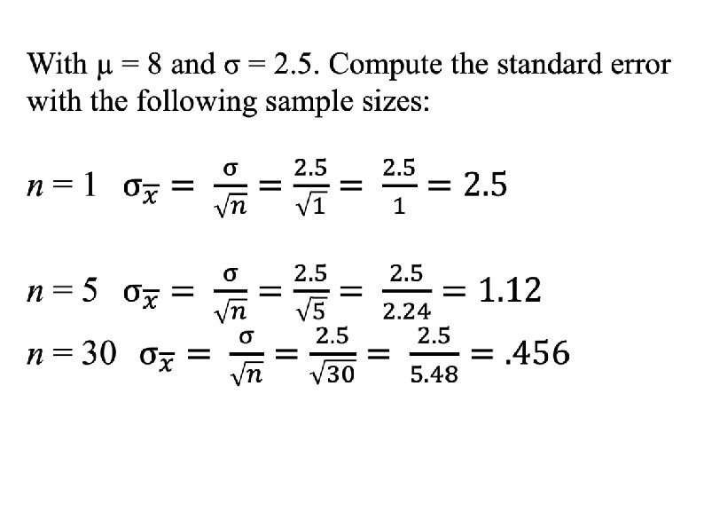
Standard deviation of the sampling distribution where σ = the standard deviation for the population n = the sample size

Standard Error of the Mean Standard error of the mean (σ ( x ) = Standard deviation of the sampling distribution of means How much the means in the distribution of means deviate from the mean of the population of individuals

Error Terms

Standard errors

The Z-Test : Hypothesis-testing with a single sample & σ2 is known Comparison distribution: Sampling distribution of means. Distribution to which you compare your sample’s mean to see how likely it is that you could have selected a sample with a mean that extreme, if the null hypothesis were true.

The Z Test

Example A person says that she can identify people of above average intelligence with her eyes closed (n = 20). STEP 1. Reframe question into a research and null hypothesis about populations. Population 1: People chosen by woman with her eyes closed (THIS IS THE SAMPLE) Population 2: People in general (Comparison Distribution, KNOWN)

Research Hypothesis (H 1): Those chosen are more intelligent Population 1 > Population 2 Population 1 has a higher mean intelligence than population 2 Null Hypothesis (H 0): Those chosen are not more intelligent Population 1 = Population 2 or µ 1 = µ 2 Population 1 does not have higher mean intelligence than population 2 or µ 1 > µ 2

STEP 3. Determine the Cutoff Sample score on the comparison distribution at which the null hypothesis should be rejected (p <. 0001). If, H 0 is true, an IQ score this extreme would be unlikely. . 01% probability (top. 01%), Z needed is 3. 719 50% -. 01 = 49. 999% ------>3. 719

If there is less than a 5% chance of a result as extreme as the sample result if the null hypothesis were true, then the null hypothesis is rejected. When this happens, the result is said to be. If there is greater than a 5% chance of a result as extreme as the sample result when the null hypothesis is true, then the null hypothesis is retained. This does not necessarily mean that the researcher accepts the null hypothesis as true—only that there is not currently enough evidence to conclude that it is true.

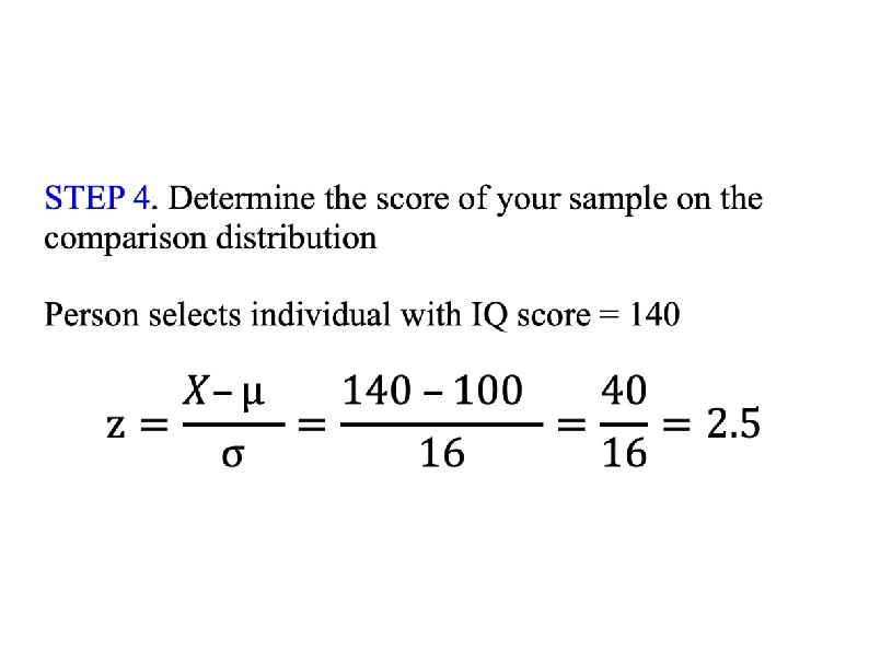
STEP 4. Determine the score of your sample on the comparison distribution Person selects 20 individuals; IQ score = 140

Step 5. Compare the scores obtained in Step 3 and 4 to decide whether to reject the null hypothesis Score on 4 (Z = 11. 17) vs. score on 3 (Z = 3. 719) Conclusion: Reject H 0: Research hypothesis is supported

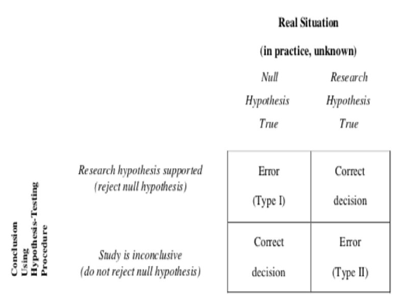
Decision Errors When the right procedures lead to the wrong decisions In spite of calculating everything correctly, conclusions drawn from hypothesis testing can still be incorrect. This is possible because you are making decisions about populations based on information in samples. Hypothesis testing is based on probability.

Hypothesis Testing Principle A person says that she can identify people of above average intelligence with her eyes closed. Is this true? 1. Define Populations & reframe hypotheses about populations Population 1: People chosen by woman Population 2: People in general (Known) H 1: µ 1 > Population µ 2 H 0: µ 1= µ 2 2. Characteristics of the comparison distribution Known normal distribution with µ = 100; σ = 16

TYPE I ERROR α 3. Determine the Cutoff Sample scores on the comparison distribution (criterion) at which the null hypothesis should be rejected (p =. 5) 50% probability (top 50%), Z needed is 0 A 30% Probability (top 30%)? Z =. 524

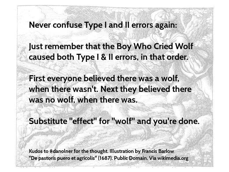
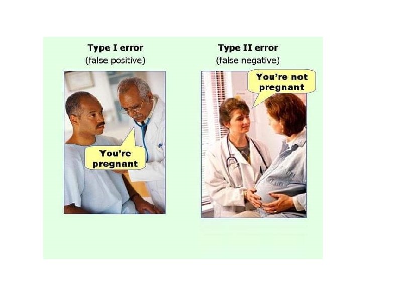
Type I (α) Error Rejecting the null hypothesis when the null hypothesis is true You find an effect when in fact there is no effect. A Type I error is a serious error as theories, research programs, treatment programs, and social programs are often based on conclusions of research studies. The chance of making a Type I error is the same as the significance level. If the significance level was set at p <. 01, there is less than a 1% chance that you could have gotten your result if the null hypothesis was true. Reduce chance of making a Type I error by decreasing significance level (e. g. , p <. 001).

Outcomes of Hypothesis Testing Type I error Reject the null hypothesis when it is correct. Saying there is a difference when there is not a difference We are rejecting a true null hypothesis. Accepting a research hypothesis when in fact it is not true

Type II Error ( ß). Not rejecting HO when it is false. Accepting HO when it is false. Saying there is not a difference when in fact there is a difference Why? Because the critical value (p <. 001) may be too extreme or low, and maybe sample representative. There maybe a difference but p value to low.

Type II Error With a very extreme significance level, there is a greater probability that you will not reject the null hypothesis when the research hypothesis is actually true. concluding that there is no effect when there is actually an effect The probability of making a Type II error can be reduced by setting a very lenient significance level (e. g. , p <. 10).

Relationship Between Type I and Type II Errors Decreasing the probability of a Type I error increases the probability of a Type II error. The compromise is to use standard significance levels of p <. 05 and p <. 01.

Type II (ß) Error With a very extreme significance level: Greater probability to not reject H 0 when the H 1 is actually true. Concluding that there is no effect when there is actually an effect Reduce Type II error by increasing p-value (e. g. , p <. 10)

Acceptance Area Rejection Area

Acceptance Area Rejection Area

Acceptance Area Rejection Area

Acceptance Area Rejection Area

Type II Error a Very High Price to Pay for Theory building: Sometimes we may abandon a particular good theory because of a small p value. Practical applications of a particular treatment Which one to use? Control Type I error by using small p (. 0001) Control Type II error by increasing p (. 2 or. 3) Use conventional values: . 01 and. 05.

Relationship Between α and β Errors Decreasing the probability of a Type I error increases the probability of a Type II error. The compromise is to use standard significance levels of p <. 05 and p <. 01.

One- and Two-Tailed Tests One-Tailed Test: A directional hypothesis: it predicts a direction of result. Also called a one-tailed test: hypothesis test looks for an extreme result at just one end (high or low end) of the curve. Psychic (high end) Stres-reduction-method example (low end)

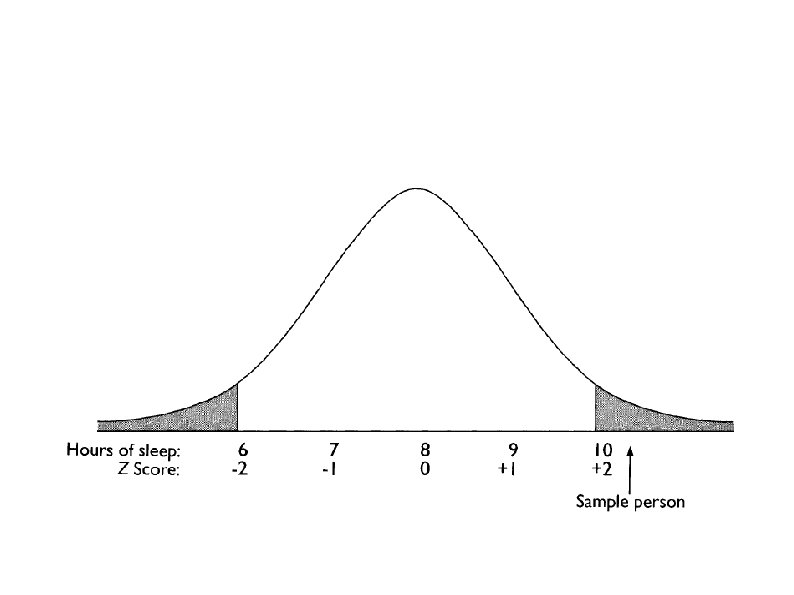
Two-Tailed Tests Experimental treatment will make a difference: Two-tailed test (non directional): Doesn't sayhow high or how low. Extreme results: Either extreme or tail (a lot or a little sleep) would make us reject the Ho Example: A polluting substance accidentally put in the water in a particular region may be suspected to affect the part of the brain that controls sleep, but it is not known whether it will increase or decrease amount of sleep.

Non-directional hypothesis: polluting substance to affect sleep BUT no direction of effect specified. In setting the cutoff for rejecting H 0 p <. 05) value divided between the two tails. 05/2 =. 025 or 2. 5% at each side. To be significant, score more extreme than if a onetailed test

One-Tailed or Two-Tailed Tests Use a one-tailed test when you have a clearly directional hypothesis (Theory Driven) Use a two-tailed test when you have a clearly non-directional hypothesis (Don't know which way). With a one-tailed test, if the sample score is extreme—but in the opposite direction—the null cannot be rejected. Often researchers will use two-tailed tests even if the hypothesis is directional (As protection!)

When to Use One-Tailed or Two. Tailed Tests Use a one-tailed test when you have a clearly directional hypothesis. Use a two-tailed test when you have a clearly nondirectional hypothesis. With a one-tailed test, if the sample score is extreme—but in the opposite direction—the null cannot be rejected. Often researchers will use two-tailed tests even if the hypothesis is directional.

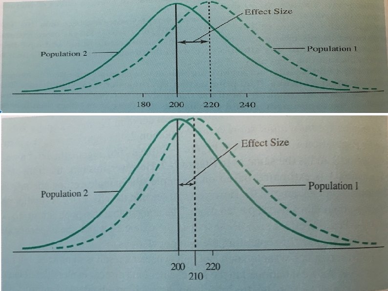
Effect Size Suppose that for Step 4: µ = 210 Still significant at p < =. 05 (Z = 1. 64) BUT a Score of 210 is less than 220 An effect can be statistically significant without having much practical significance.

Hartley & Heredia

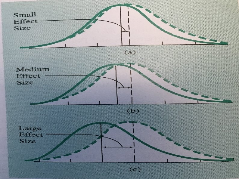
Effect Size A measure of the difference between populations. Tells us how much something changes after a specific intervention. Indicates the extent to which two populations do not overlap. how much populations are separated due to the experimental procedure With a smaller effect size, the populations will overlap more.

Formula for Calculating the Effect Size µ 1= µ receiving experimental manipulation (SAMPLE) µ 2 = µ (comparison distribution) σ = SD of the population of individuals A negative effect size would mean that the mean of µ 1 is lower than the mean of µ 2

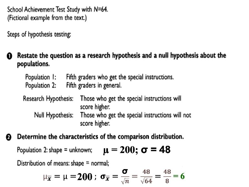
Calculating the Effect Size For the sample of 64 fifth graders: best estimate of µ 1 = x 1 = 220. µ 2 = 200, σ2 = 48. Indicating that the effect of the experimental manipulation (e. g. , reading program Special instructions) increased the reading level scores by. 42 SD’s.

Effect Size Conventions

General Importance of Effect Size Knowing effect size of a study lets you compare results with effect sizes found in other studies (even when the other studies have different population SDs). Knowing the effect size lets you compare studies using different measures, even if the measures have different means and variances. Knowing what is a small or a large effect size helps you evaluate the overall importance of a result. A result may be statistically significant without having a very large effect.

General Importance of Effect Size Meta-Analysis a procedure combining results from different studies, even results using different methods or measurements This is a quantitative rather than a qualitative review of the literature. Effect sizes are a crucial part of this procedure.

Statistical Power Probability that the study will produce a statistically significant result if the research hypothesis is true (controlling TYPE II ERROR) When a study has only a small chance of being significant even if the research hypothesis is true, the study has low power. When a study has a high chance of being significant when the study hypothesis is actually true, the study has high power.

Hartley & Heredia

Hartley & Heredia

Statistical Power Statistical power: how many participants are needed. Helps you make sense of the results that are not significant or results that are statistically significant but not of practical importance. Determine power: Power software package or a power calculator. Power can also be found on a power table.

What Determines Power of a Study? The statistical power of a study depends on: how big an effect the research hypothesis predicts effect size (Small, Medium, Large) how many participants are in the study sample size other factors that influence power include: significance level chosen (p <. 001 low power) whether a one-tailed or two-tailed test is used the kind of hypothesis-testing procedure used

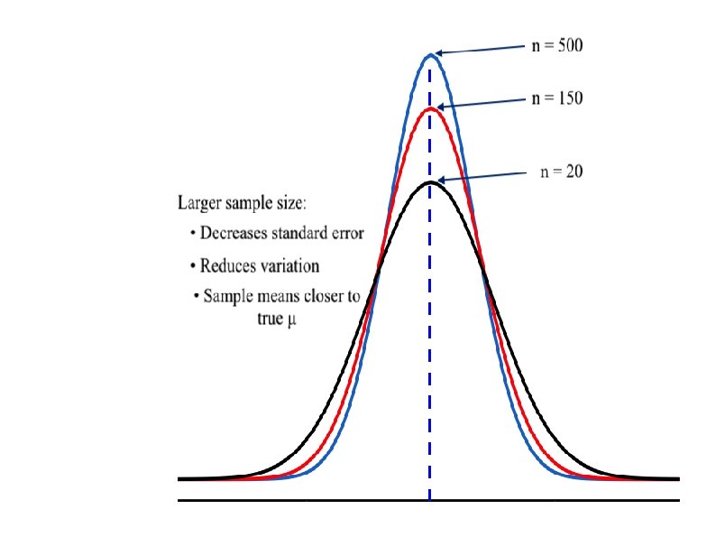
Sample Size The more people in the study, the greater the power. The larger the sample size, the smaller the standard deviation of the distribution of means becomes (Decrease Sampling error). The smaller the standard deviation of the distribution of means, the narrower the distribution of means—and the less overlap there is between distributions leading to higher power.

Other Influences on Power Significance Level Less extreme significance levels (e. g. , p <. 10) mean more power because the shaded rejection area of the lower curve is bigger and more of the area in the upper curve is shaded. More extreme significance levels (e. g. , p <. 001) mean less power because the shaded region in the lower curve is smaller. One- vs. Two-Tailed Tests Using a two-tailed test makes it harder to get significance on any one tail. Power is less with a two-tailed test than a one-tailed test.

Statistical vs. Practical Significance Possible for a study with a small effect size to be significant. Results may be statistically significant, but may not have any practical significance. e. g. , if you tested a psychological treatment and your result is not big enough to make a difference that matters when treating patients

Statistical vs. Practical Significance Evaluating the practical significance of study results is important when studying hypotheses that have practical implications. Whether a therapy treatment works, whether a particular math tutoring program actually helps to improve math skills, With a small sample size, if a result is statistically significant, it is likely to be practically significant. In a study with a large sample size, the effect size should also be considered.

Role of Power When a Result is Not Statistically Significant A nonsignificant result from a study with low power is truly inconclusive. A nonsignificant result from a study with high power suggests that: the research hypothesis is false or there is less of an effect than was predicted when calculating power

Significance in Sample Size in Interpreting Research Results If result is statistically significant and N is small, the result is important (Large effect size) If the result is statistically significant and the sample size is large, the result might or might not have practical implications (TOO MUCH POWER). If result is not statistically significant and the N is small, the result is inconclusive. If result is not statistically significant and the N is large, the research hypothesis is probably false.

Effect Size and Power in Research Articles often mention effect size. Effect size is a crucial factor in meta- analyses, and thus is almost always reported in metaanalyses. Power is sometimes discussed when evaluating nonsignificant results.